

Introduction
Theoretical Background
Permeability Data
Permeability Models for Production-induced Reservoir Compaction
Modelling Methodology
Effects of Initial Permeability and Looping Time Step on the Model
Model Validation by Field Data
Summary and Conclusions
Introduction
Fluid transport in oil and gas reservoirs is generally controlled by reservoir permeability (David et al., 1994; Zhu and Wong, 1997). Permeability estimation is one of the most difficult problems in modeling how fluid percolates in a specific lithological and tectonic settings. The reasons are, firstly, that permeability commonly varies by more than 10 orders of magnitude in geological materials (Freeze and Cherry, 1979); secondly, that this parameter is sensitive to pressure and temperature, which are often complicated by tectonic and metamorphic processes (Fyfe, 1978); and thirdly, that in situ permeability and laboratory measured values in sampled reservoir rocks can be significantly different due to the possible presence of mesoscopic scale fractures (Brace, 1980). Moreover, permeability is intimately related to the pore-space geometry, which is usually represented by porosity (Zhu and Wong, 1997). In sedimentary rocks, porosity and permeability are stress-dependent parameters, therefore, a fundamental understanding of porosity and permeability evolution due to stress is important in many rock mechanics applications (David et al., 1994; Zhu and Wong, 1997).
Fluid extraction from petroleum reservoirs generally causes a decrease in pore pressure, which results in a change of stress condition and reservoir compaction (Chin et al., 2001). Permeability and porosity of the reservoir rocks vary due to stress change and in turn affects the production of oil and gas. Such a looping process from fluid extraction, through changes in pore pressure and stress, to reservoir compaction and permeability evolution, and towards fluid extraction again makes it difficult to estimate pore pressure and production rate conditions in the reservoir. In this study, we investigate three different permeability models typically assumed in the literature to check which of these are most pertinent to predict reservoir process during production. These permeability models are: (1) the most simplistic constant and invariable permeability during production, (2) reduced permeability under uncoupled stress-pore pressure condition, and (3) reduced permeability with stress-pore pressure condition coupled. Variable permeability model has been shown to work generally better from the fully coupled geomechanics and fluid flow analysis (Chin et al., 2001). Thus, we include the model (3) in this study to gain more insight into the effect of stress change on permeability evolution. As permeability affects the way pore pressure changes during production, as well as the extracting rate, it is important to find the most realistic permeability evolution models among the three.
In this paper, we first study permeability behavior corresponding to stress of 5 types of sandstones, namely, Adamswiller, Boise, Darley Dale, Rothbach and Berea, then apply the stress-permeability relationship onto the aforementioned 3 permeability models to describe pore pressure distribution and permeability evolution due to fluid extraction in a sandstone reservoir. Finally, we utilize 2 sets of field data to test the results given by the 3 permeability models in order to find the best fit.
Theoretical Background
For typical reservoir rocks (i.e. sandstones), the evolution of porosity and permeability has been studied extensively through laboratory compaction experiments under various stress conditions (Walder and Nur, 1984; Rice, 1992; David et al., 1994). Fig. 1 shows typical laboratory compaction test configuration, in which rock specimen is loaded by axial maximum principal stress (σ1) and lateral confining pressure (σ2 = σ3). Compaction of the specimen is measured using axial and radial linear variable differential transformers (LVDTs). Pore pressure in the rock specimen is independently applied through water inlet. The difference between external compressive stress and internal pore pressure is usually referred to as effective stress, which has strong impact on permeability of the rock. Such stress conditions are designed to simulate stress and pore pressure conditions in a petroleum reservoir. As the external compressive stress in a reservoir is normally driven by tectonic origin and the overburden, neither of which change dramatically during lifetime of petroleum production, the effective stress changes mostly due to a change in pore pressure during petroleum production. Generally, oil and gas production would result in pore pressure drawdown in the reservoirs, consequently increasing effective stress. The increased effective stress would cause reservoir compaction (i.e., reduction of porosity and permeability) by pore collapse and micro-crack closure (Brace, 1980; David et al., 1994).

Although permeability evolution due to compaction of reservoir rocks is well-known for many kinds of different sandstones, there is no unique relationship that unifies permeability-stress and permeability-porosity correlations for all kinds of sandstones. However, typical forms of such relations are given by (Brace, 1980; Yale, 1984; Nelson and Anderson, 1992; Zhang et al., 1994):
| $$K=K_0\left(\frac\phi{\phi_0}\right)^\alpha$$ | (1) |
| $$K=K _{0} 10 ^{\beta ( \phi - \phi _{0} )}$$ | (2) |
| $$K=K _{0} e ^{- \gamma (P _{eff} -P _{0} )}$$ | (3) |
where, K is permeability of rock; Peff is effective confining pressure; f is porosity; initial permeability (K0) and initial porosity (ϕ0) are defined as the permeability and porosity of the sample at initial confining pressure P0, respectively. ɣ is effective stress sensitivity coefficient, α is porosity sensitivity exponent and β is porosity sensitivity coefficient. David et al. (1994) determined values of α and ɣ for 5 different sandstones (Adamswiller, Fontainebleau, Berea, Rothbach, and Boise). The α values range between 4.6 and 25.4, and those of ɣ range between 6.6 × 10⁻³ and 18.1 × 10⁻³ MPa-1, indicating that permeability evolution associated with changes in confining pressure and porosity is significantly distinct for different sandstones. In an attempt to define a unified permeability and compaction relationship for various sandstones, we compile compaction test data from the literature (Zhu and Wong, 1997), which is described in the next section.
Permeability Data
The collected data include confining pressure, porosity and permeability of 5 types of sandstones (Adamswiller, Boise, Darley Dale, Rothbach and Berea). We plot the data in the form of permeability versus effective confining pressure in Fig. 2. All tests were performed at a nominal pore pressure of 10 MPa. Table 1 gives details about petrophysical description of the studied sandstones including grain size, initial porosity and modal analysis. The porosities of those 5 sandstones vary in a wide range from 14.5% up to 35%. The confining pressure applied to those sandstones was up to 540 MPa, by which the samples compact to induce a decrease in permeability by more than 3 orders of magnitude.
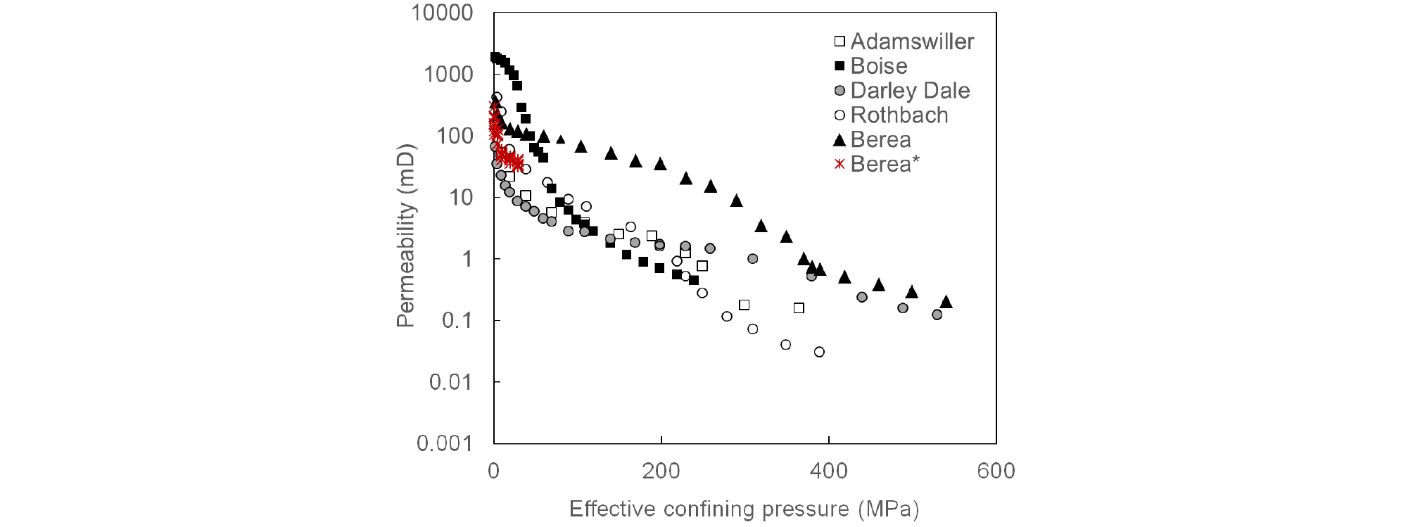
Table 1. Physical description of the studied sandstones
David et al., 1994; Heap et al., 2009.We also run permeability measurements in Berea sandstone to check the repeatability of the data, which is marked as Berea* in Fig. 2. Our permeability measurements are conducted under effective confining pressure ranging from 1 to 30 MPa using the triaxial compression apparatus shown in Fig. 1. In our test, a pair of axial LVDTs and a radial LVDT are used to measure the sample’s axial and lateral strain, respectively, during the compaction process in order to measure porosity change while water is pumped through the sample by a syringe pump. Pore pressure is maintained at 0.1 MPa.
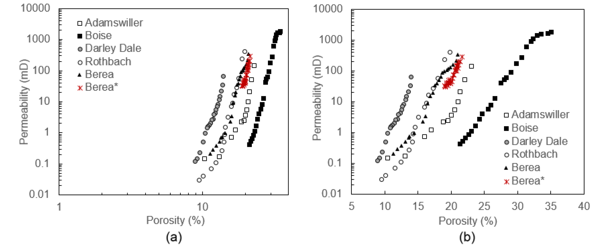
The permeability is also plotted as a function of porosity in a semi-log plot and a log-log plot (Fig. 3a and 3b). Fairly good linear trends are observed in both cases, which means that permeability can be expressed either by an exponential function or by power function of porosity (Walder and Nur, 1984):
As mentioned earlier, different sandstones exhibit distinct compaction parameters, ɣ, α and β. We calculate these parameters for all sandstones in the dataset in order to find a proper way to replace these parameters with a common one that represents all the sandstones tested. Note that we only calculate ɣ for effective confining pressure less than 50 MPa, since we believe that this amount of pore pressure change is sufficient to cover typical reservoir depletion due to petroleum production. Consequently, our calculated ɣ is relatively higher than that calculated by David et al. (1994), because permeability is generally more sensitive under the early stage of pressure increase.
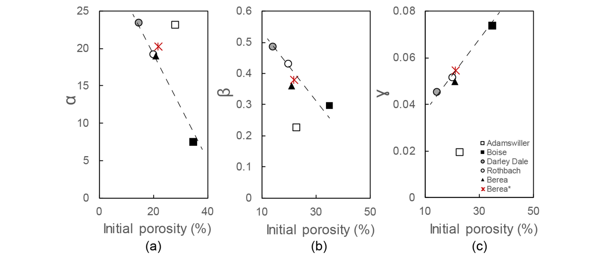
Interestingly, we find good relations between initial porosity (ϕ0) and each of α, β and ɣ (Fig. 4). Particularly, Boise sandstone, exhibiting the highest initial porosity, indicates highest value of ɣ and lowest value of α and β, while Darley Dale sandstone, exhibiting the lowest initial porosity, shows much lower value of ɣ and highest value of α and β. In other words, higher initial porosity sandstone is more sensitive to pressure but less sensitive to porosity change. Linear correlations between initial porosity (ϕ0) and each of α, β and ɣ are given as:
| $$\alpha =-0.7937 \phi _{0} +35.635$$ | (4) |
| $$\beta =-0.0085 \phi _{0} +0.5811$$ | (5) |
| $$\gamma =0.0014 \phi _{0} +0.0246$$ | (6) |
| $$K=K_0\left(\frac\phi{\phi_0}\right)^{-0.7937\phi_0+35.635}$$ | (7) |
| $$K=K _{0} 10 ^{(-0.0085 \phi _{0} +0.5811)( \phi - \phi _{0} )}$$ | (8) |
| $$K=K _{0} e ^{-(0.0014 \phi _{0} +0.0246)(P _{eff} -P _{0} )}$$ | (9) |
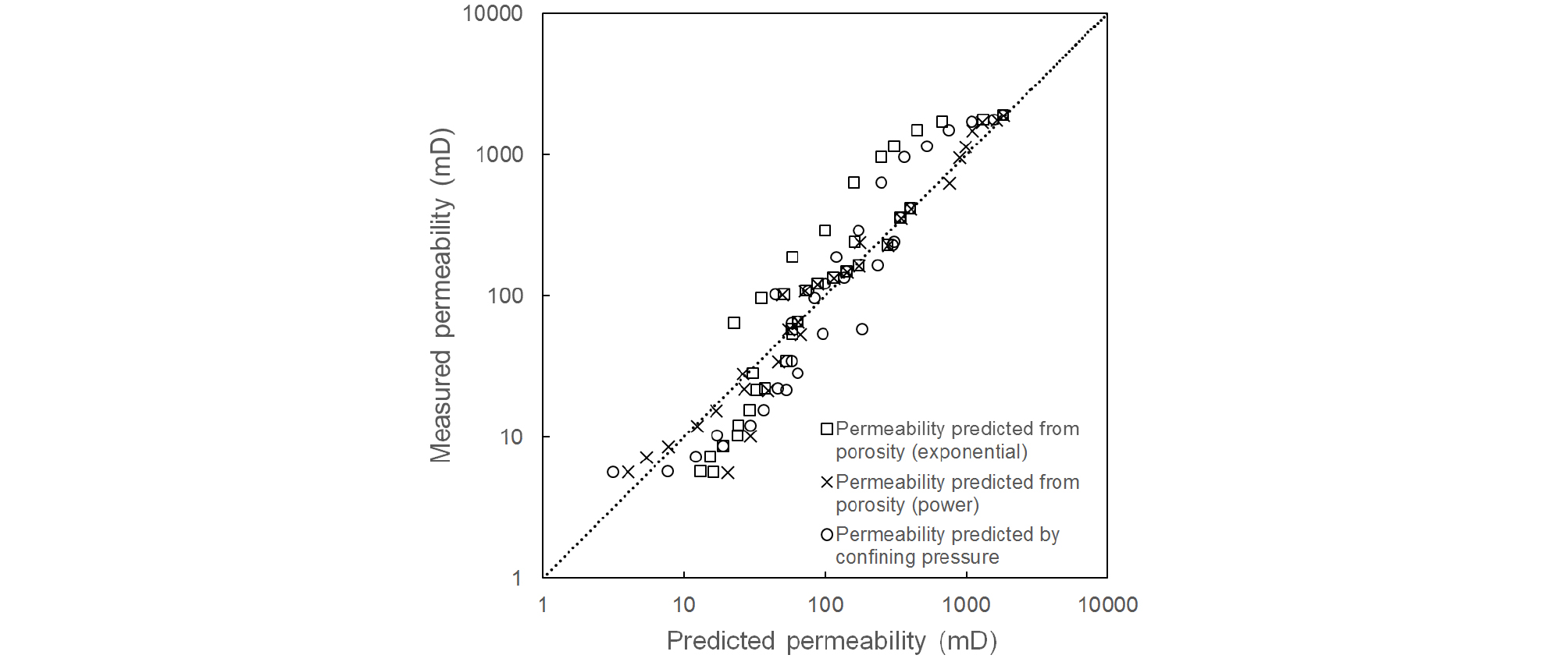
Eqs. (7)~(9) enable the prediction of permeability evolution due to compaction (i.e., due to increasing effective confining pressure or decreasing porosity), where sensitivity coefficients (α, β or ɣ) are expressed in terms of initial porosity. We plot permeability prediction from effective confining pressure and from porosity of the studied sandstones versus the laboratory measured permeability (Fig. 5). The difference between predicted and laboratory measured permeability is less than 1 order of magnitude.
Permeability Models for Production-induced Reservoir Compaction
Modelling Methodology
We use a simple cylindrical reservoir model, in which a vertical production well is at the center (Fig. 6). We assume that the fluid is single-phase oil and the reservoir is isotropic and homogeneous, with an initial pore pressure of Pi and an initial permeability of K0 before production. Details of model parameters are given in Table 2. When oil is produced through the vertical well, reservoir pressure begins to drop, which forms an area called “drainage area” where pressure depletion creates a pressure funnel (Fig. 6). Drainage area is marked by dash in Fig. 6, which represents a no-flow boundary, beyond which the reservoir pore pressure is unaffected and remains its initial pore pressure (Pi). Pe is the pressure at the no-flow boundary, at the distance re from the wellbore center. The lowest pressure value of the pressure funnel is Pwf, which is equivalent to bottom-hole pressure; K is reservoir horizontal permeability; h is reservoir thickness; µ is fluid viscosity; B0 is oil formation volume factor; and rw is wellbore radius (Guo et al., 2007; Ahmed, 2010).
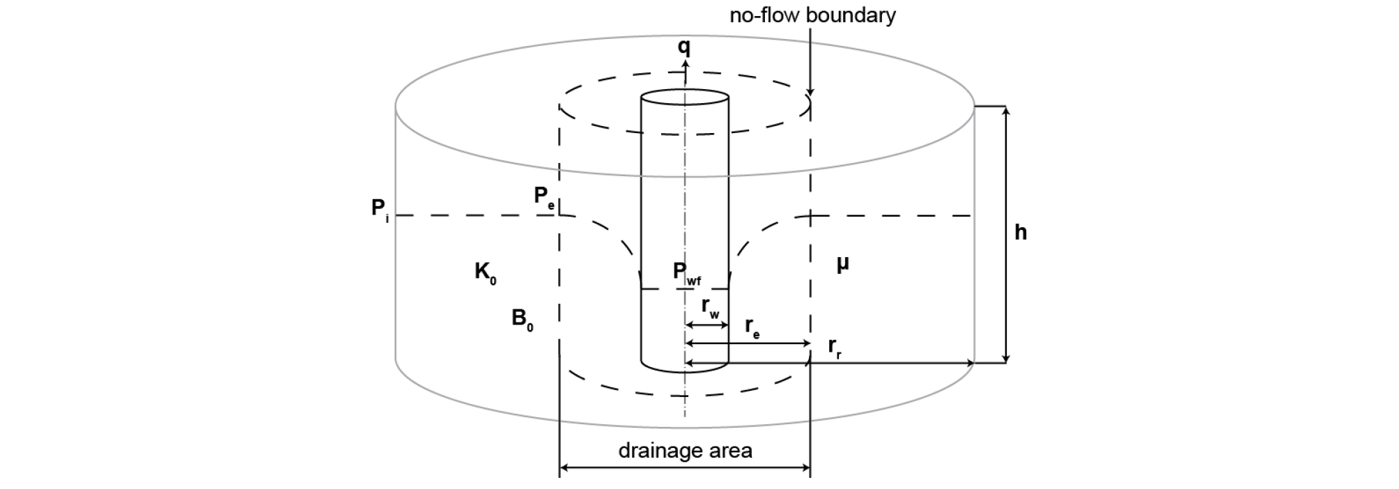
Table 2. Reservoir properties and well properties for modelling
We use the pressure diffusion equation to model fluid flow:
| $$\frac{dP} {dt} = \frac{K} {\phi \mu C _{t} R} \frac{d}{dR}\left( R \frac{dP}{dR}\right)$$ | (10) |
where, P is pressure, R is radial distance from the well center, t is time, K is permeability, f is porosity, Ct is total compressibility and m is fluid viscosity (Kruseman et al., 1994).
At the initial condition when pressure is in its virgin state, P(R, t = 0) = Pi. Given that the flow rate in the drainage area is constant at q, and the pressure at no flow boundary remains Pi, the solution for the diffusion equation can be obtained in the form of an integral solution (Wu and Pruess, 2000), which is also known as the Theis’s solution:
| $$P(R,t)=P_i+\left[\frac{q\mu}{4\pi Kh}\right]\left[-E_i\left(-\frac1{4t_D}\right)\right]$$ | (11) |
| $$t _{D} = \frac{Kt} {\phi \mu C _{t} r ^{2}}$$ | (12) |
We assume three different permeability models: (1) the most simplistic constant and invariable permeability, (2) reduced permeability under uncoupled stress-pore pressure condition, and (3) reduced permeability with stress-pore pressure condition coupled. The Model 1, which assumes that permeability remains constant during production, simply considers the loss of pressure during production as the only factor that affects the production rate. Therefore, the looping process consists only 2 stages: fluid extraction decreases the pressure in the reservoir in a diffusion form and pressure depletion in turn reduces the extraction rate. For the Model 2 and Model 3, we involve the effect of permeability reduction in the looping process, which starts from fluid extraction, through changes in pore pressure and effective stress, to reservoir compaction and permeability evolution, and towards fluid extraction again. However, the Model 2 does not consider pore pressure-stress coupling, so the amount of pore pressure depletion will be the amount of effective stress increase. In the Model 3 where pore pressure-stress coupling is applied, the external stress changes associated with pore pressure drawdown. For layered reservoir formations where the formation lateral extent is sufficiently larger than thickness, externally exerting horizontal stress would actually change with a change in pore pressure. This process, also known as coupling between pore pressure and stress, is expressed by (Hillis, 2000):
| $$\frac{\triangle \sigma _{h}} {\triangle P _{p}} = \alpha \frac{1-2 \nu } {1- \nu }$$ | (13) |
where, σh is externally exerting horizontal stress, α is Biot constant and n is Poisson’s ratio for rock formations. If we use typical values for α (= 1) and n (= 0.25), Eq. (13) gives a value of 0.67. Therefore, under this coupled condition, oil production results in decreases in both pore pressure and external stress.
With the reservoir and well properties presented in Table 2 and workflow for each model presented by Fig. 7, the 3 models are applied to calculate pore pressure distribution around the well during 50 days of producing (Fig. 8). The Model 1 assuming constant permeability obviously predicts the least amount of drawdown with pore pressure condition highest among the three models investigated. After 50 days of producing, the pore pressure around the borehole drops by ~3.5 MPa, while that at 100 m distance from the well drops by less than 1.5 MPa. Model 2 estimates the largest amount of pore pressure drawdown and thus the lowest pore pressure condition, with pore pressure around the borehole drops by more than 5 MPa and that at the boundary drops by more than 2 MPa. Model 3 shows slightly higher pore pressure condition than Model 2 because stress-pore pressure coupling process reduces the effective stress increase due to pore pressure depletion.
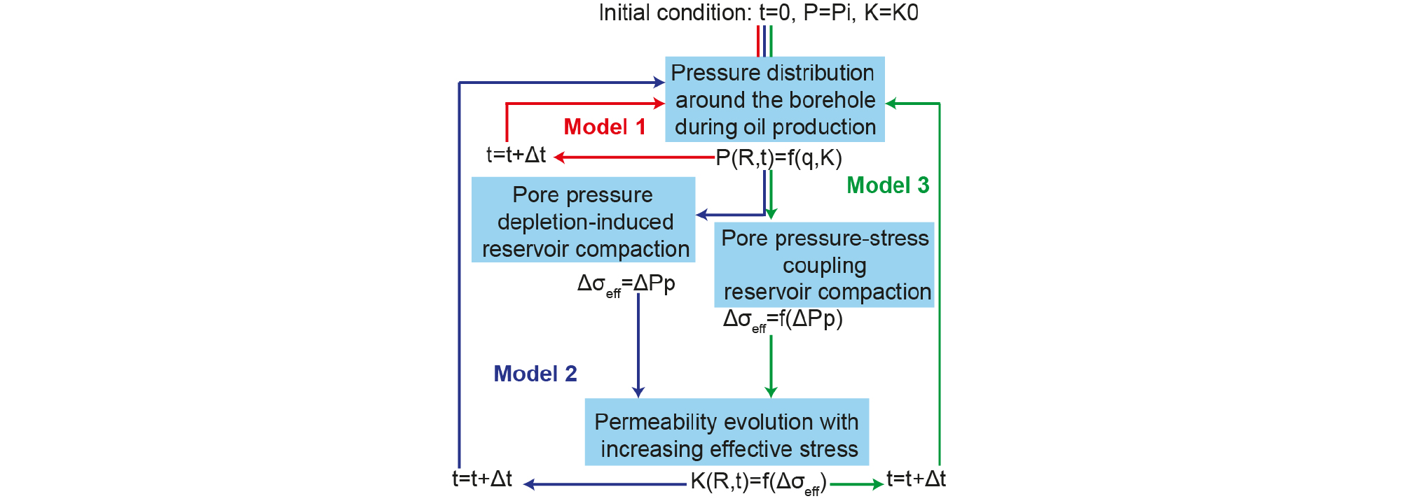
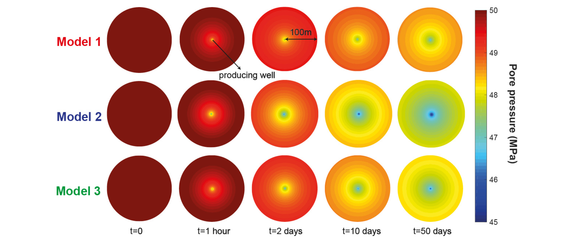
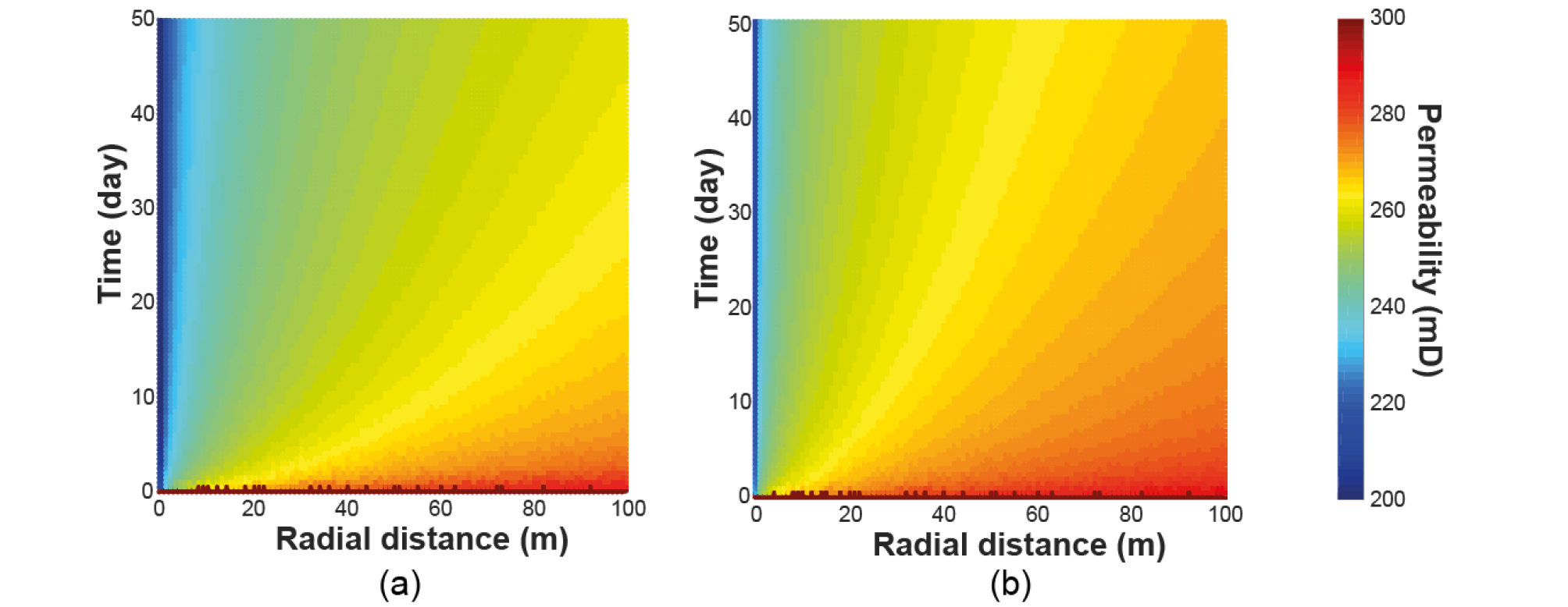
Fig. 9 shows permeability evolution during production with time and space estimated by the Model 2 and 3. It is evident that permeability decreases from the reservoir boundary to the well in terms of space, and from the beginning of production to the 50th day in terms of time.
Effects of Initial Permeability and Looping Time Step on the Model
The two factors that may affect the models are (1) initial permeability K0, which is the permeability of the reservoir before production, and (2) looping time step Δt - the period after which the pore pressure, stress and permeability are updated. Fig. 10a illustrates how pressure at the boundary of the model (R = 100 m) declines with time. It is evident that in high initial permeability case (K0 = 600 mD), pore pressure at the boundary of the model drops less than 1 MPa, and there is almost no difference among three models. However, in relatively low permeability case (K0 = 100 mD), the difference in pore pressure drawdown between Model 1 and 2 is as great as ~25% after 50 days of production, while that between Model 2 and 3 is ~10%. This can lead to 2 conclusions. First, higher initial permeability reservoir has its pore pressure drop less than relatively low initial permeability reservoir with the same production level; second, the lower the initial permeability of the reservoir is, the more significantly the predicted pore pressure by the 3 models will be different.
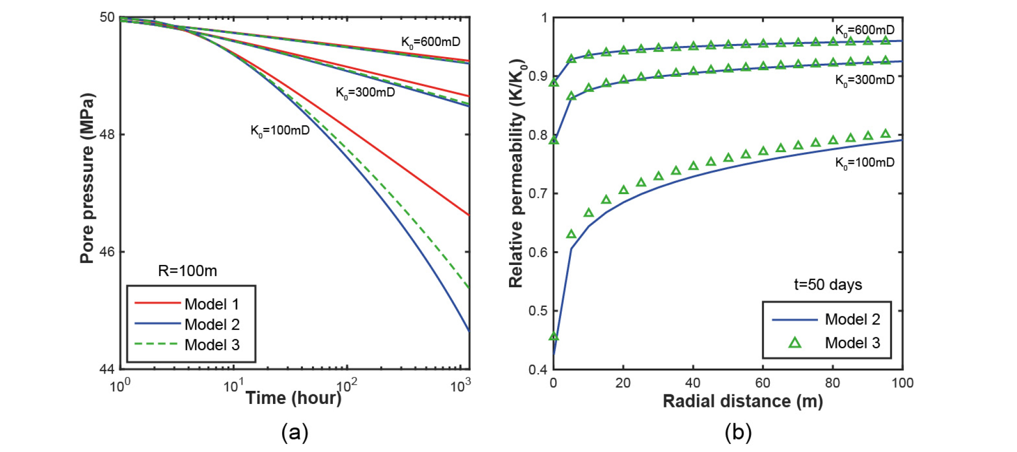
Not only pore pressure but permeability evolution also depends on the reservoir initial permeability. Fig. 10b shows that permeability curves predicted by Model 2 and Model 3 are almost the same in the case of high initial permeability reservoir (K0 = 600 mD and K0 = 300 mD) but quite different in the case of K0 = 100 mD. Moreover, higher initial permeability reservoir has its permeability decrease less than low initial permeability reservoir with the same production rate, as permeability in case of K0 = 100 mD dramatically drops after 50 days of production especially within the area around the borehole (~50%).
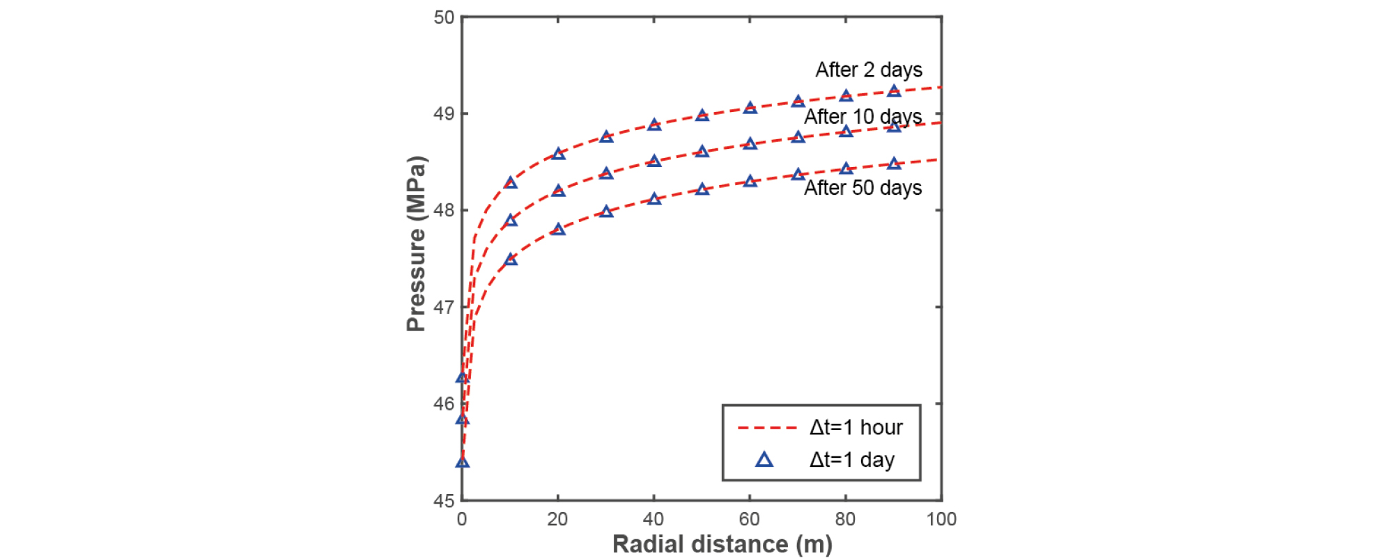
Choosing different time step can change the total running time for the models significantly. Thus, we test our model with 2 different time step value: 1 hour and 1 day. Obviously, the number of looping calculations in the case of 1 hour is 24 times more than the case of 1 day. Therefore, we want to confirm whether choosing smaller time step gives better pressure and permeability prediction so that it would be worth. However, we find that time curves derived from the different time steps almost the same (except for the very first 2 days) indicates that time step do not have remarkable impact on the results given by our models (Fig. 11).
Model Validation by Field Data
In an attempt to validate the 3 models investigated in the present study, we compare the model results with actual production data from Stanko et al. (2015) and Ink et al. (2007). Reservoir properties are taken from the literature and initial pore pressures are calibrated to fit a sandstone reservoir.
We use the following equation derived from Darcy’s law for a reservoir under pseudo-steady state (the pressure at any point of the reservoir decreases at the same rate over time), which is frequently utilized in petroleum production engineering (Ahmed, 2010):
| $$q=7\pi10^{-6}\frac{Kh(P_e-P_{wf})}{B_0\mu_0\left(\frac12ln\frac{r_e}{r_w}+S\right)}$$ | (14) |
where, Pwf : bottom hole pressure (MPa)
Pe : pressure at the no-flow boundary (reservoir pressure) (MPa)
re : drainage radius (m)
q : production rate (m3/s)
µ0 : viscosity (Pa.s)
B0 : fluid formation volume factor
K : reservoir horizontal permeability (mD)
f : porosity, fraction
h : reservoir thickness (m)
rw : wellbore radius to the sand face (m)
S : skin factor
We use the results of our 3 models (pore pressure at the no-flow boundary with time and permeability evolution with time) to apply to the equation above to predict production rate, given that bottom-hole pressure is known. Predictions made by the 3 models and the real production data are shown in Fig. 12. It is obvious that Model 3 estimates the field data fairly well while the Model 1 and the Model 2 do not really match the real production data. For example, the Model 1, in which permeability is assumed to remain constant, significantly overestimates the actual production rate. This is because permeability of the reservoir is believed to decrease due to compaction as fluid is extracted from the reservoir. Model 2 generally underestimate actual production rate data, which is attributed to overestimation in the degree of reservoir compaction. In this case, the increasing effective stress acting on the reservoir might not be equal to the amount of decreasing pore pressure, but relatively lower. For the reasons, the Model 3 which include both permeability evolution during production and stress-pore pressure coupling shows best estimation out of the three models compared.

Fig. 12.
Comparison between production rate predicted by 3 permeability models and field production rate data in 2 cases. Field data are employed from Ink et al. (2007) (a) and Stanko et al. (2015) (b).
Because the three models give relatively same prediction when the reservoir is porous and permeable (initial permeability K0 > 500 mD), we try to test our models in the condition of relatively low initial permeability (K0 ≤ 100 mD) so that we can see clearly the gap between the models’ results. The results show that the Model 3 shows best prediction, which means that reduced permeability with stress-pore pressure condition coupled may be the most proper assumption for permeability modelling.
Summary and Conclusions
We attempt to derive an equation that can be used to predict permeability for sandstones either from porosity or from confining pressure, in order to predict permeability evolution and further to assess production rate in sand reservoirs. We use a widely utilized equation that relates permeability to an exponential function of effective stress to unify permeability-effective stress relationships for five different sandstones (Berea, Adamswiller, Bose, Rothbach and Darley Dale) that were compiled from the literature. To further check the re-peatability of the data, we also measure permeability evolution in Berea sandstone under varying confining pressures. We derive a unified equation that can fit the compiled permeability and pressure data for all the sandstones tested.
We use the diffusion equation to describe how pore pressure changes and distributes during oil production, with different permeability conditions: (1) constant permeability, (2) reduced permeability under uncoupled stress-pore pressure condition, and (3) reduced permeability with stress-pore pressure condition coupled. We compare the pressure distribution as well as permeability evolution estimated by 3 models and investigate 2 factors that may affect the results given by the models such as initial reservoir permeability and looping time step. We find that initial permeability does affect the results of the 3 models as lower initial permeability makes the difference between the 3 models more severe. In contrast, looping time step does not have considerable effect on the models’ results.
We utilize 2 sets of field production data to test our models in the condition of relatively low initial permeability so that the models give considerably different results. Using the pore pressure and permeability evolution prediction from the models, we were able to calculate the production rates and compare with the real data. We find that the Model 3 estimates the rates which match well with the real data, while the Model 1 and the Model 2 respectively overestimate and underestimate the rate. While previous studies have found that a variable permeability model works better compared to a constant permeability model (Chin et al., 2001), it can be concluded in our study that incorporation of the coupling process in the permeability modelling might be even more accurate and important especially for tight reservoir which has low initial permeability.
