Introduction

The variability of sporadic precipitation, short-term runoff ephemeral streams, loss of water due to high evapotranspiration makes water supply tough, especially, in the arid and semi-arid regions. Moreover, recently, climate change and variability are exacerbating the problem (Lasage et al., 2013; Ryan et al., 2016). To tackle these water challenges, there have been several mechanisms proposed and some of them are implemented all over the world including weather modification, water harvesting, desalination, and water reuse (Walsh, 1965; Hutchinson et al., 2010). Among these, water harvesting using sand dam has been implemented largely in arid and semi-arid regions (Lasage et al., 2007).

A sand dam is a flow barrier built across small or medium size sandy rivers to accumulate sand upstream of it and store water for longer use or enhancement of the groundwater recharge (Sivils and Brock, 1981). The presence of sand dam makes the flow to have lower velocity (but sufficient enough to wash fine particles (Hoogmoed, 2007)) and the bed load will have a chance to be deposited and raise the bed elevation gradually up to the dam height. Therefore, raising the riverbed level by accumulating the sand and increasing the groundwater storage is the principal goal of sand dam construction (Hoogmoed, 2007). To achieve this goal the design and construction of a sand dam should be based on the appropriate site selection. The basic requirements are: it needs to be environmentally friendly, the natural flow system should not be affected, downstream riverbed should be protected from erosion and the dam should be protected from the flood at the riverbanks (Ryan and Elsner, 2016). These requirements are mainly related to the construction of appurtenant structures such as a spillway, wing wall, and erosion protection.

When the sand accumulates on the upstream side of the dam the water will have a chance to be trapped in the sand protected from evaporation and at the same time, it will have a longer time to infiltrate and join the groundwater below the river bed (Hoogmoed, 2007). The excess water, especially during the rainy season, is stored. The water stored in the sand can be used in the dry period, usually by digging a few centimeters from the surface (scoop hole) or by installing pumping wells at the riverbanks.

The ability of sand to control evaporation make it preferable for the storage of water in the arid or semi-arid areas (Sivils and Brock, 1981). The productivity and effectiveness of the sand dam to store water for long period has a direct relationship with the depth of the accumulated sand (Bleich, 1983). The specific yield of the sand is also the determining factor in the storage capacity of the sand dam (Hanson and Nilsson, 1986). The size of the sand dam is mostly not greater than 6 m on 10 to 100 m wide gorges (Aerts et al., 2007). Sand can store up to 40% of its volume (Quinn et al., 2018). Moreover, as the water goes down through the sand it gets filtered (slow sand filter system) so that if the river flow is not significantly affected by pollutants the stored water can be used for domestic, irrigation, and animals without any treatment (Ertsen and Hut, 2009; Hatem, 2016).

In the recent or coming climate change resulted water scarcity sand dam can be a solution (Aerts et al. 2007). Especially if the area has good aquifer it can enhance the recharge of groundwater and the extractable amount of the groundwater can be increased much larger.

If the river is perennial river the accumulated sand will simply increase the river bed from its original position to the top of the sand. Even if the sand dam is a kind of flow barrier structure, it is usually designed in a way to preserve the environmental flow in the river. So that there will be no high storage of water like any other reservoirs and the water required for ecological balance is kept safe. As mentioned above the construction of the sand dam has some criteria to fulfill. Some countries have long time experience and have matured principles and guidelines for the construction of the sand dam.

Sand dams are also built for the purpose of harvesting, riverbed crossing in the rural area, sand and rehabilitate gullies. To rehabilitate the erosion-damaged rivers in rural areas serious of small sand dams are constructed and soil is accumulated and the river bed is recovered. In a similar way, if the river has ‘construction quality’ sand people construct a sand dam and just for collecting the sand.

In general, as several studies show that this method of reserving excess water is cost-effective and simple but essential technique, especially in the arid and semi-arid regions (Ryan and Elsner, 2016; Lasage et al., 2007; Sivils and Brock, 1981). Besides its simple storage of water in the sand for the dry period use through scoop holes, recently, the sand dam is becoming a way of increasing the water table and the amount of abstractable groundwater (El-Hames, 2012). However, the studies which relate the groundwater and sand dam are limited. Moreover, all the studies are case studies. It is not easy to see the effect of the sand dam on the aquifer in the sand dam area.

This work focus on the investigation of the relationship of the sand dam and the groundwater potential using numerical models. The aquifer dimension, hydrogeological properties, and the different scenarios are all ideal designed by the modeler in a way which enables to visualize the phenomena clearly.

Sand Dam Experiences

Even though the sand dam is not documented separated from the subsurface dam (sand dam and underground dam) the history may go back to Sardinia in Roman times and ancient African civilization (Hanson and Nilsson, 1986). Recently, India, Japan, Brazil, Pakistan, Kenya, and Ethiopia are some of the examples for the sand dam using countries (Villani et al., 2018; Nishgaki et al., 2004). There are also experiences in America using sand dam for reserving water for wildlife and livestock since 1973 and reported that the sand dam has great potential to improve wildlife in an economical way (Sivils and Brock, 1981; Bleich, 1983). As the studies show mostly the application of sand dams in almost all countries is in the arid and semi-arid areas (Sivils and Brock, 1981; Jadhav et al., 2012).

Case studies of sand dam development in Kenya, especially in the Eastern region are reported by several researchers and organizations (Lasage et al., 1981; Aerts et al., 2007; Ertsen and Hut, 2009). In this region, 500 sand dams with a height ranging from 1 to 4 m above the surface are built and contributing to the economic growth of the community (Ertsen and Hut, 2009). The community in Kitui, Eastern Kenya uses water from the sand dam for commercial products such as horticulture, brick production, and others.

Ethiopia has been implementing a sand dam in large and small-scale project packages (Tuinhof et al., 2012). As the reports show the sand dam for water storage have been developed in several parts of the country and it is reported as successful (Lasage et al., 2013). Farmers benefit from the sand dam by irrigating and increasing the agricultural productivity in the Ethiopian dry season (Villani et al., 2018). The impact of the sand dam on the hydrology of the area also investigated and implicated that the sand dam has a positive impact on the hydrology and the environment of the areas. In this country, the role of the sand dam in securing water supply under climate change is also investigated and made positive conclusions (Lasage et al., 2013).

In general, nowadays, the sand dam is more common in Africa, especially in the east and west African countries than the other part of the world (Villani et al., 2018). The relative simplicity and efficiency of sand dam technology are renovating attention in the rest of the world.

Groundwater Flow Modeling

A modular finite-difference groundwater flow model, MODFLOW (McDonald and Harbaugh, 1988) is employed to simulate the effect of the sand dam on the water table. MODFLOW is widely applied and acceptable model for groundwater flow simulation.

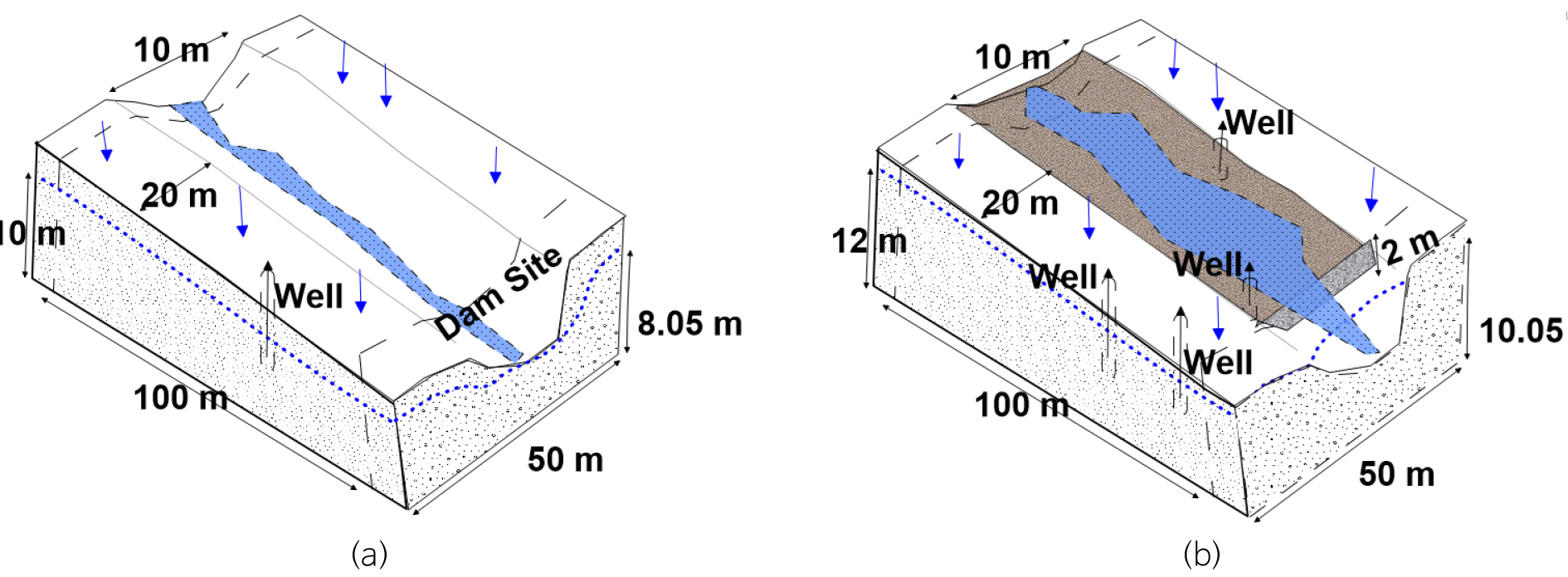
Two models are developed. The first model represents a pseudo-natural small aquifer in a semi-arid. The water table is deep in the area due to a low riverbed elevation compared to the land surface. The second model considers a sand dam, which adds a sand layer with a thickness of 2 m on a 10 m wide gorge. Assuming the first model takes only the saturated section, in the second model we have increased negligible thickness at the riverbanks to prevent splicing of mathematical layers due to the addition of the sand layer. The dimensions and properties of the two models are tabulated in Table 1.

Table 1. Dimensions and hydrogeological characteristics of the models

Since the model dimension is small, all the parameters are assumed spatially uniform. To select the hydrogeological properties, the pumping and recharge rates are fixed first and simulated in steady state and transient state condition by varying, mainly, the hydraulic conductivity (K) and specific yield until the water table get closer to the riverbed. These model results are taken as the base condition of the aquifer and the reported results are not included in this paper.

In addition to the hydrogeological properties, to define the aquifer system numerically, the discretization of the model area and identifying the boundary conditions are necessary. The selected model area is discretized into 40 cells in the x-direction, 9 cells in the z-direction, and 10 cells in the y-direction, which resulted in 3600 active cells. Then the top and bottom of the cells of the river are modified to 2 m lower than the cells at the riverbanks, gradually, to make the model expressive of the concept explained in Fig. 1.

Fig. 1.

Schematics of sand dam hydrology and basic components (Modified from Borst and Haas, 2006).

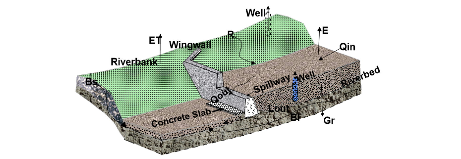
For the transient state, the simulation time is discretized into stress periods and time steps, which represent only the change in recharge and groundwater abstraction rates, the temporal change of other boundary conditions, is kept constant to see the effect of pumping wells on the water table. The total simulation time is 365, with 12 stress periods and 365-time steps. The first stress period is with no pumping of groundwater and the other 11 stress periods are with different pumping rates.

The model geometry and boundary conditions are depicted in Fig. 2. The initial head is assumed to equal to the top layer of each mathematical layer. Considering the size of the model and availability of minimum flow in the river, the entrance and exit of the river are assumed to be a constant head boundary with a head value of the upstream 10 and 12 m, at the downstream 8.05 and 10.05 m before and after the construction of the sand dam respectively. A river hydraulically connected to the aquifer with the uniform flow with a depth of 0.25 m is incorporated into the model. Uniformly distributed surface recharge temporarily ranging from 2.83E-05 to 1.7E-04 m/day is applied.

Fig. 2.

Dimensions and boundary conditions of the models: (a) before the construction of the sand dam, (b) after the construction of the sand dam.

After all the hydrogeological properties are fixed by several trial simulation, the first simulation was the steady state to check the stability of the model, once more, and to get the initial head for the transient state simulation. Then to see the effect of different groundwater abstraction rates on the water table fluctuation the transient simulation is performed.

In the first model, a single layer with 1m/day horizontal hydraulic conductivity and 0.02 specific yield are considered. One pumping well is used at the bank of the river with pumping rate varying from 1 to 8.5 m³/day.

The second model is developed by taking the same aquifer setting of the previous model and adding the sand layer on the riverbed. In this model size, the thickness of the sand layer on the riverbed has a negligible difference from upstream to downstream. Therefore, the depth is increased in a small difference from upstream to the dam site to a maximum depth of 2 m at the dam site. Horizontal flow barrier (HFB) with low hydraulic conductivity is used at the dam site. HFB is a package which enables to model the effect of flow barriers such as sheet piles slurry, and trenches (https://www.xmswiki.com/wiki/GMS:HFB_Package#HFB_Package_Dialog).

The properties of the new sand layer are tested by running the model several times. The stability of the model is better in the high hydraulic conductivity compared to the previous model. The hydraulic conductivity of this new layer is set to be 150 m/day.

Results and Discussion

The water table changes and the amount of extractable water, without a significant effect on the water level, are identified by running the models several times with random water pumping rates. The water budget of the entire model at selected stress period is computed using USGS ZONEBUDGET (Harbaugh, 1990). ZONEBUDGET is a USGS code integrated with MODFLOW to read cell-to-cell flow data and compute the water budget of sub-regions of the model. The results are presented in the form of cross-sectional view, graphical plots, and in tabular forms.

Groundwater Flow without a Sand Dam

The results in the idealized pseudo-natural aquifer system (the first model) are shown in Fig. 3. It shows the water table and velocity vectors at a section across the pumping well, in the stress period 2, time step 1 (water pumping started). The groundwater flow is with gentle water table slope from upstream to downstream having a maximum and minimum head of 9.95 m and 8.1 m, respectively. The effect of groundwater abstraction is not noticeable and the water table elevation is almost similar to the static water table.

Fig. 3.

A cross-sectional view of the model before the construction of a sand dam at 1 m³/day pumping rate.

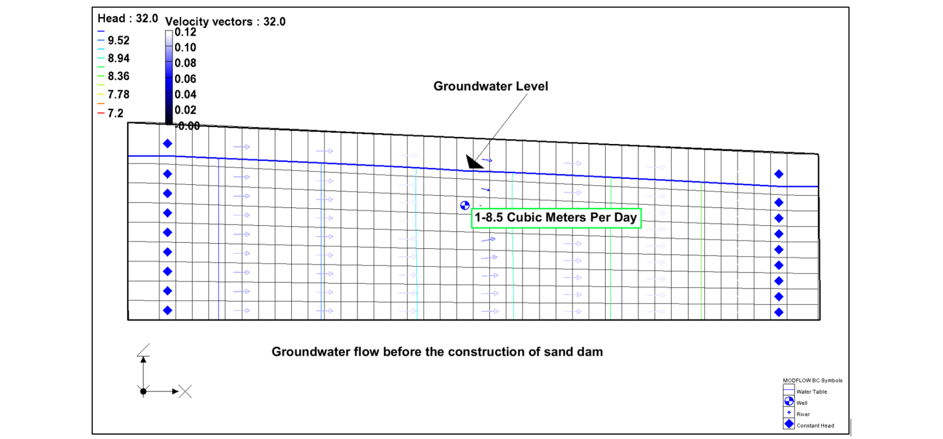
Table 2 shows the water budget of the first model at stress period 2, time step 1. The inflow-outflow system is dominated by the constant head, the contribution of river leakage and recharge are trivial. In this simulation time, the leakage is from the river to the aquifer only, no leakage to the river. Even if the outflow system is higher than the inflow, the water table looks stable. Therefore, assuming 1 m³/day pumping don’t show a significant water table change a new higher pumping rate is added into the model. In this way, several trial simulations are performed until the water table around the pumping well creates a cone of depression.

Table 2. Flow budget of the model at time step1 stress period 2

The model results at the maximum pumping rate of 8.5 m³/day are also shown in Fig. 4. Compared to the previous results, the water table decreased significantly, especially around the pumping well. The minimum head is 7.01 m, which is around 1 m less than the previous results minimum head. When the pumping rate increases from this specified rate the model get unstable and could not converge.

Fig. 4.

Cross-sectional view of the model before the construction of a sand dam at 8.5 m³/day pumping rate.

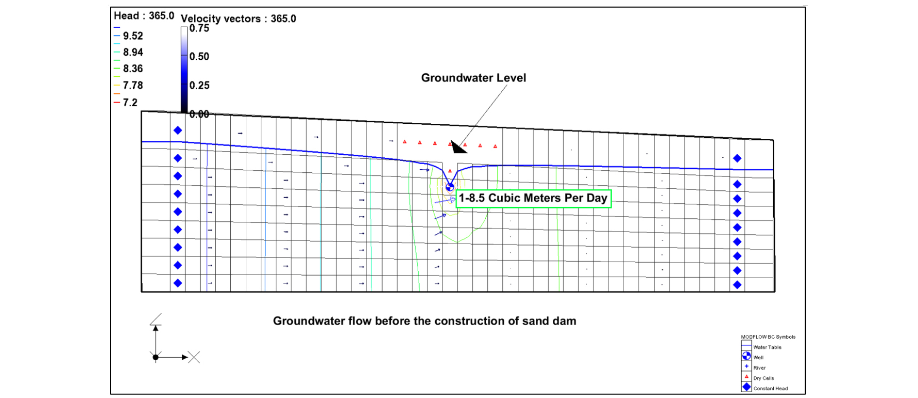
The groundwater table is always less than the riverbed elevation, which implies that the groundwater abstraction rate is always greater than the aquifer recharge rate. Therefore, in the pseudo-natural aquifer, the groundwater abstraction rate should be less than 8.5 m³/day.

Moreover, as the flow budget (Table 3) shows while the inflows in terms of constant head, river leakage, and recharge are constant, storage as inflow from the previous stress period shows a big difference compared to the results of the model at stress period 1.

Table 3. Flow budget of the model at time step 365 stress period 12

In general, the total water inflow to the system at 1 m³/day and 8.5m³/day, abstraction rates, are 8.64 m³/day and 12 m³/day respectively. From this, the aquifer recharge from the rainfall and river leakage is 0.36 m³/day. Therefore, even though it is possible to withdraw water upto 8.5 m³/day the amount of extractable water should be equal to the aquifer replenishment rate.

Groundwater flow with Sand Dam

When the riverbed elevated gradually to the sand dam height the water table is also increased much higher than the previous model. The water table is in this model is near to the land surface even at the riverbanks.

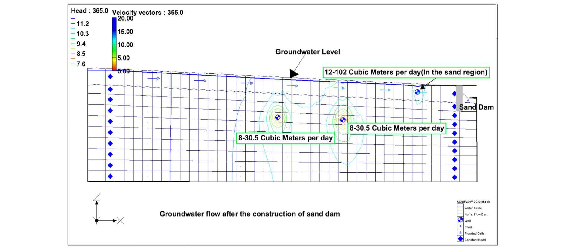
The number of pumping wells and pumping rates are increased to see the corresponding water table changes. Fig. 5 shows the water table with three pumping wells at the minimum abstraction rates of 8 and 12 m³/day. The pumping rate in the sand layer is high. In this model, the velocity vector of the sand layer is dominant and compared to the results of the first model it is high and uniform from upstream to downstream.

Fig. 5.

A cross-sectional view of the model after the construction of the sand dam at the minimum pumping rates.

Comparison of the first results of the two models reveals the groundwater storage inflow from the previous simulation time is 0.869 m³/day and the second model is increased to 13.1 m³/day and other terms show an increase. The pumping rate in the first trial is also increased to 28 m³/day, which was 1 m³/day in the first model.

As we can see in the Fig. 6, this pumping rate has a negligible effect on the water table, though it is higher than the pumping rates in the first model. Moreover, in addition to the water leakage to the river, which was not there in the first model, the leakage to the aquifer is decreased. The water table is higher than the riverbed in some sections and lower in other sections of the model. This aquifer property is more a representative of semi-arid region aquifer.

Fig. 6.

Model result of an aquifer with the sand dam at the end of the simulation.

In this model interestingly as the hydraulic conductivity of the sand layer increases the amount of extractable water and water table increases. However, the focus of this study is limited to the comparison of the groundwater flow before and after the construction of a sand dam. Therefore, a single hydraulic conductivity with moderate value but much higher than the hydraulic conductivity of the pseudo-aquifer layer is used for the sand layer.

Interestingly the aquifer response to an increase in pumping rates after the construction of the sand dam is active in all the flow term. As we can see from both Tables 4 and 5 as the pumping rates increase the inflow from the river and the constant head boundary shows incensement. Therefore, the presence of sand dams in the area is a balancing mechanism for both river flow and groundwater flow.

Table 4. Flow budget of the second model at time step1 stress period 2

Table 5. Flow budget of the second model at time step 365, stress period 12

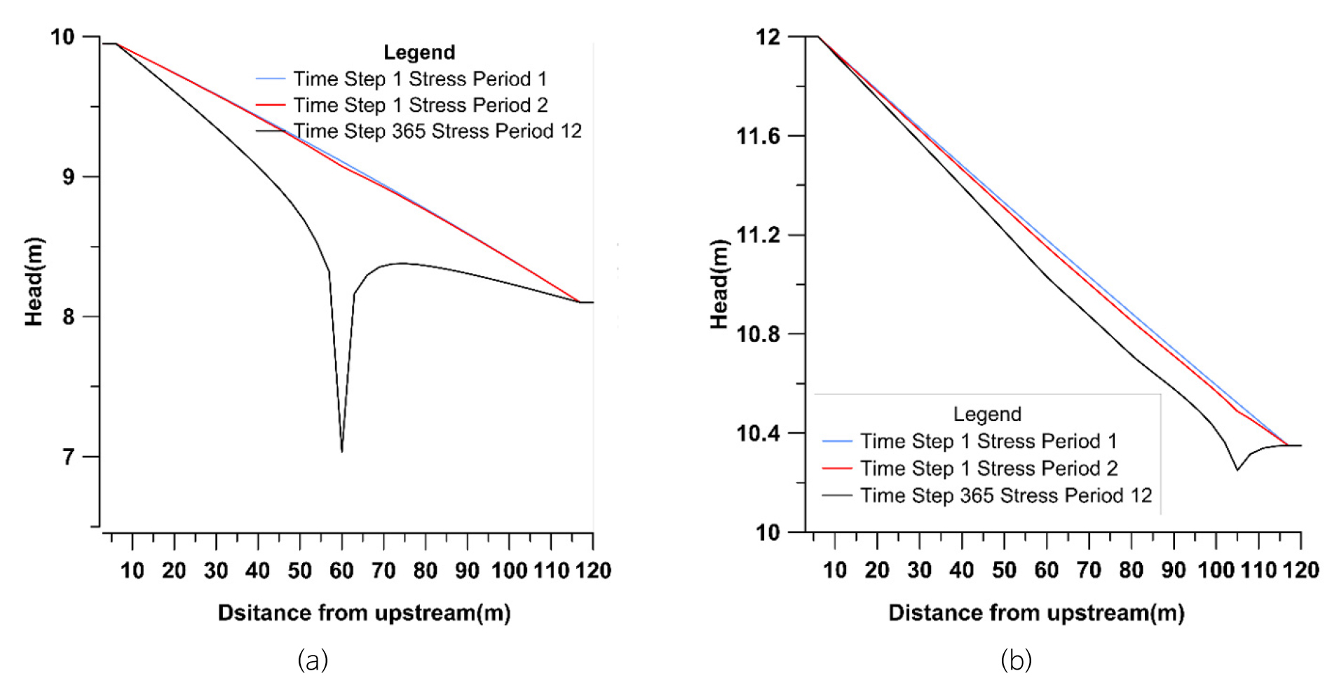
To show the clear image of the effect of the sand dam on the water table fluctuation of the level is plotted on the same graph. Fig. 7 shows the water table of the two models in the static condition, at a minimum and maximum pumping rate. Fig. 7a is before the construction of the sand dam. In this Fig., the difference between the maximum and minimum head is almost close to 3 m with a maximum change of more than 2 m. Fig. 7b is an aquifer with a sand dam and the difference of the minimum and the maximum head is less than 2 m with a maximum change of 0.25 m. This comparison shows that the water table of an aquifer with the sand dam is more stable at high groundwater abstraction rates.

Fig. 7.

Comparison of the water table in the model area: (a) before sand dam (pseudo-natural aquifer), (b) after the construction of the sand dam.

Conclusion

The effect of the sand dam on groundwater flow is investigated using numerical models. Two models, assuming semi-arid region aquifer, are developed. The first model is a pseudo-natural aquifer with a low river flow, conceptualized to simulate groundwater flow before the construction of the sand dam. Using this model, different pumping rates are tried, to check the amount of exploitable groundwater without affecting the water table significantly. The second model, which has a 2 m sand thickness riverbed, is used to see the effect of the sand dam on the groundwater. The comparison of the model results and the rate of groundwater abstraction rate with the corresponding change of water table show that the construction of sand dam increases the amount of groundwater abstraction rate by many folds. However, the type of sand material has a significant effect on the effectiveness of the sand dam. The construction of the sand dam stored water in and facilitates the movement of the water to the groundwater so that the water table increased significantly almost equal to the level of the sand surface.