

Introduction
Method to Achieve GA Structure
Encoding
Object Function
Parent Selection
Crossover
Mutation
Population Maintenance
Cluster Exchange
Results
Conclusion
Appendix
Introduction
Water is one of our most important resources. Its use for irrigation constitutes a significant portion of global demand. Methods to supply water for large-scale agricultural irrigation have diversified, and the amounts of water used have increased. Groundwater consumption has increased particularly rapidly (Siebert et al., 2010). The extraction of groundwater from aquifers often leads to their depletion (Wada et al., 2010), as occasional high-intensity rainfall only recharges some of the taken groundwater (Thomas et al., 2016). Sustained depletion may change the environment of nearby rivers through groundwater-surface water interactions (Chang and Chung, 2015). In addition, the continued global consumption of water will intensify drought (Wada et al., 2013). To manage the risk of groundwater depletion, regulations should allow for appropriate groundwater extraction rather than its unconditional prohibition.
The management of ground water generally aims to maximize the yield from an aquifer or to minimize the cost of pumping a given amount (Wang and Zheng, 1998).
Search algorithms for optimization are often used in this field of study. A representative example is the genetic algorithm (GA), which has been utilized in many operational research problems such as the traveling salesman and airplane hub problems. It is the most popular among various evolutional algorithms that mimic biological evolution to solve extremely difficult problems (Dréo et al., 2006). McKinney and Lin (1994) provided a benchmark problem for groundwater management and solved it using the GA; before this, the use of GAs in groundwater management was uncommon. Their work was among the first to analyze the feasibility of using GAs to solve typical issues in this field of study, and utilized classical and simple GAs. Many types of linear, nonlinear, and statistical models can optimize the management of groundwater (McKinney and Lin, 1994). However, traditional methods cannot guarantee global optimal solutions. Our current work, reported here, combined the GA with numerical solution of the groundwater flow equation.
This study comprised two parts: groundwater flow calculation and the GA. The groundwater flow equation is essential for calculating the head variation along the Euclidean distance x. The head was used to evaluate one of the constraints. A MATLAB code segregated into two subroutines was used. The first subroutine (subroutine 1) was the flow equation, which calculated the flow equation of groundwater. The second subroutine (subroutine 2) was the GA code.
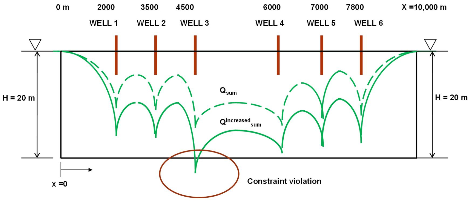
Fig. 1 depicts the problem domain. It shows the configuration of the aquifer and six potential pumping well locations. Even though the study area can be described as an unconfined aquifer, the flow-governing equation of a hypothetical confined aquifer was used to test the GA process. To simplify groundwater modeling, an unconfined aquifer can be assumed to be confined when it simulates steady-state condition. Hill (2006) reported that this simplification reduced computing time without reducing accuracy. The left and right boundaries were considered as constant head boundaries set as 20 m, equal to the depth of the aquifer. The aquifer measured 10,000 m × 20 m, and the cell grid size was 10 m × 20 m. The domain comprised 1000 columns and 1 row. The hydraulic conductivity was 50 m/day. The storage coefficient was not considered because the head was calculated only under steady-state conditions. The domain comprised six wells, each with a different pumping rate; their locations were not evenly distributed to prevent a symmetric result.
The following notations are used herein.
System parameters
H : Saturated depth of the aquifer
Qi : Pumping rate of well i
Qsum : The sum of the amount of well pumping
Qincreased sum : The sum of the increased amount of well pumping
hxi : Head at coordinate x by well pumping i
hx : Integrated head at coordinate x by superposition
rj : Coordinate of jth node, which is the same as the distance of the jth node from the left boundary
di : Distance of well i from the left boundary
p : Value of the penalty function.
ps : Population size
Decision variables
Qi : Pumping rate at well i
Constraint
hi : Head at location of well i
Method to Achieve GA Structure
Encoding
This study’s objective is to maximize the overall pumping rate, which is the sum of each well’s pumping. Therefore, the pumping rate of each well, Qi, is a decision variable in the GA. The first step is to create a genotype from the phenotype. To encode a decision variable as a genotype, McKinney and Lin (1994) used a traditional binary structure. Binary encoding is the most widely used method in the GA, because a binary string is easy to code and manipulate. McKinney and Lin (1994) originally used three-digit binary substrings corresponding to 10 wells. The individual substrings were then concatenated into a string of 30 binary digits. This study compared two different encoding methods: 1) binary strings and 2) real numbers. Binary string encoding randomly generated a 14-digit (rather than three-digit) binary string for each decision variable. The longer binary strings allowed more-precise value changes. Real number encoding encoded each decision variable, Qi, as a real number generated randomly in the range of 0~16,000 m3/day. Each of the real numbers was then concatenated into a string of six genes corresponding to six wells.
Object Function
The object function is the summation of the well pumping rates. The drawdown must be within 20 m, and individual pumping rates must be in the range of 0~16,000 m3/day. The values of water elevation in the constraint set were predicted by a groundwater simulation model. The amount of any constraint violation is multiplied by a weight factor and added to the fitness value as a penalty. The pseudo equation of the object function (a) and the mathematical form (b) are shown below.
where, fi is the fitness value, M is the total number of constraints, ji is the weight factor, and di is the amount of violation.
To evaluate the fitness function, the constraint h, which is termed the head or water level, must be evaluated by solving the groundwater flow equation for well pumping. Adopting a radial flow based on polar coordinates (instead of Cartesian x-y coordinates) allows a simpler governing equation to be used rather than a 2D flow equation. The governing Eq. (1) for well pumping is as follows:
The head at each well location was calculated based on the above governing equation. It was used as a constraint factor to determine the penalty function and well pumping rates. The equation links the groundwater hydraulic head in the confined aquifer (h, [m]), the coordinate in the aquifer domain (r, [m]), the storativity of the confined aquifer (S), and the transmissivity (T, [m2/day]). In this study, the head profile was evaluated only for steady-state conditions. Therefore, the Eq. (1) was transformed to the following:
When the head variation of each well was calculated, the head was integrated by superposition.
where, i = 1, 2 … number of wells.
Finally, the fitness term was evaluated by verifying the constraint violation. McKinney and Lin (1994) used a penalty function as the sum of the weight factor multiplied by the amount of violation of the jth constraint. This study investigated two new penalty functions. The first assigned a constant value to the penalty if the constraint violated the specified condition. The constant value was determined empirically by trial and error; it was set here to 3000. The second penalty function used a dynamic value that had the same range as the decision variables. The value provided to the code was p = random number [0, 1] × 3000.
Parent Selection
We adopted a tournament strategy. For the tournament selection process, four designs were selected from the current population. Subsequently, the two winning designs from this tournament were subjected to the crossover operator.
Crossover
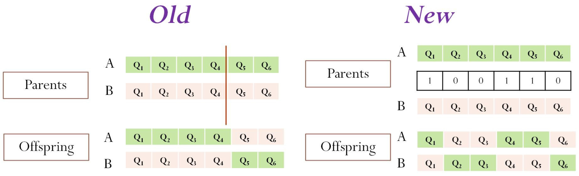
McKinney and Lin (1994) used the crosscut strategy (“Old” in Fig. 2 shows an example). The parents are selected by tournament, and crossover is performed at a single, randomly selected point. Single-point crossover was performed on each mated pair with a crossover probability. These two new strings were considered as children and formed members of a new population. This study employed multipoint crossover based on binary selection: a binary number mask was randomly generated with a length equal to the solution length. If the binary digit is 1 at the nth position, offspring 1 and 2 maintain the nth genes of parents 1 and 2, respectively. Conversely, if the binary digit is 0 at the nth position, offspring 1 and 2 maintain the nth gene of parents 2 and 1, respectively.
Mutation
After crossover, the offspring are mutated. McKinney and Lin (1994) flipped one bit of an offspring with probability 1/(population size). This study attempted real-value mutation. For mutation, the selected gene’s real value was randomly generated between 0 and 16,000. This is the same step as used to generate the initial solution of the decision variable. Dejong’s (1975) suggestion of inverse population size for mutation probability was not adopted here, because crossover between real number strings cannot create new values for the decision variable. To create a diverse population, a higher mutation probability (pm) of 0.3 was assigned here.
Population Maintenance
Our experiments applied elitism by placing the best chromosome at each generation. Generally, the iteration repeats these steps until convergence or the maximum number of generations is reached. McKinney and Lin (1994) stopped the iteration after the GA solution converged to the maximum value of 58,000 m3/day; the best solution was obtained after 10 iterations. However, Wang and Zheng (1998) obtained a better solution after a longer iteration. Therefore, we did not terminate the process even if some degree of convergence occurred. Instead, we detected the best solution for each generation until the iteration proceeded to the maximum number. We expected a better optimal solution after performing a sufficiently large number of iterations. The maximum number of generations was set to 200, which was greater than that of Wang and Zheng (1998).
Cluster Exchange
Cluster exchange is another form of crossover (see Fig. 3). This operator is executed after one iteration ends. We compared two types of cluster exchange. The concept of “cluster” originated from the hub problem. A cluster is defined as the set of decision variables that are allocated to a given hub (Ernst and Krishnamoorthy, 1996). This study modified the cluster concept to fit the groundwater problem. Each decision variable, Qi, behaved as a spoke in the hub problem. Each cluster comprised three decision variables. The selection of a decision variable depended on the domain location, which was expressed as an array in MATLAB. The entire code of the problem comprised two subroutines. The first (subroutine 1) was a flow equation used to calculate the flow equation of groundwater. The second (subroutine 2) was the GA code.
The distance array (di) is an independent variable of the flow equation. It has been used to calculate the head in subroutine 1. The distance array was not observed, and hence was not used for the GA code in subroutine 2 before the cluster concept was adopted. The cluster concept used the distance array in the GA code. Individuals that were near each other were gathered into the same cluster. This study considered two clusters. All the individuals in one cluster moved to the other after each iteration. This resulted in diversity among the individuals and prevented the solution from remaining at the current local optimum during the GA’s execution.
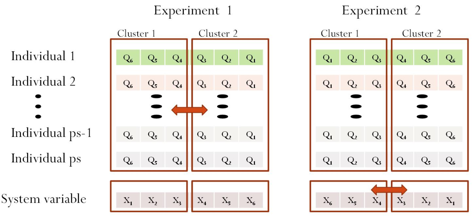
Experiment 1 used a mechanism that follows the definition of exchange between clusters: exchange between decision variables. Even though we added the “cluster exchange” operator, the best solution did not exhibit a significant improvement. The pseudo-code is shown below.
For i = 1 to ps
For j = 1 to well_number/2
Q(I,j) = Q(I,well_number/2+1-i)
End
End
The mechanism used in experiment 2 was adopted here. The concept is fundamentally identical to that of experiment 1. All decision variables (Qi) corresponded to non-decision variables (di). Array x is a system parameter that represents the coordinates of wells. In the conventional GA, the MATLAB code addresses only the decision variable for swapping and mutation. Our new approach addresses the system parameter (di) in the GA code. The pseudo-code of experiment 2 is as follows.
For i = 1 to well_number/2
x(i) = x(well_number/2+1-i)
end
Initially, Qi for all the population corresponds to xi. The exchanges between clusters indicate that Q6 corresponds to r1, Q5 to r2, Q4 to r3, Q3 to r4, Q2 to r5, and Q1 to r6 for both experiments 1 and 2. The constraint factor, h, is a function of distance and pumping rate. It can be expressed as f(Q,x). Therefore, the head profile results were h1(Q6, x1), h2(Q5, x2), h3(Q4, x3), h4(Q3, x4), h5(Q2, x5), and h6(Q1, x6) for both cases.
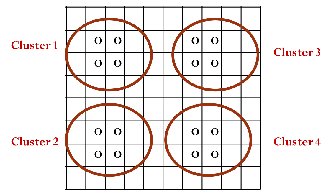
The effect of cluster heuristics is expected to be apparent in complex domains such as the 2D aquifer. Fig. 4 shows the concept of clustering at a 2D well pumping site. The decision making of a cluster depends on the Euclidean distance between individuals. The example involves 16 wells distributed over the domain. Three cluster combinations can be made if four clusters are formed and exchanged by grouping four wells. In this case, more diversity is expected to be created because a large number of clusters will increase the number of exchanges. The pseudo-code of the GA algorithm is listed in the Appendix.
Results
Table 1 compares GA operators from the original paper and this study. Their encoding, crossover, mutation penalty function, and cluster exchange all differ. Each operator was changed individually. Therefore, five different simulations were performed for these cases.
Table 1.
Comparison of GA operators
| GA operator | McKinney and Lin (1994) | This study | |
| 1 | Encoding | Binary string | Real number |
| 2 | Parent selection | Tournament selection | Tournament selection |
| 3 | Crossover | Single-point crossover | Multipoint and cluster exchange |
| 4 | Mutation | Binary flip | Random solution |
| 5 | Population maintenance | Elitism | Elitism |
| 6 | Penalty function | Number of constraints × Weight factor | Dynamic value |
| 7 | Termination | Maximum generation | Maximum generation |
Table 2 lists the parameter values used here. Each was determined empirically by trial and error. The value of the mutation probability for binary encoding (0.01) was calculated based on Dejong’s (1975) suggestion of using the inverse of population size.
Table 2.
GA parameter values
| Parameter | Initial values | |
| 1 | Population | 100 |
| 2 | Crossover probability | 0.4 |
| 3 | Mutation probability | 0.3 (0.01 for binary encoding) |
| 4 | Generation | 200 |
Table 3 lists the operators used in each case. For the GA simulation, we investigated five different cases. Case 1 was the most similar to that of McKinney and Lin (1994), the only difference being encoding: a longer binary string was created randomly to allow more precise changes. The range was consistent when compared with those of other cases. Case 5 differed from Case 2 by having a real number as a genotype. Case 3 had a modified crossover strategy. In Case 4, the penalty function was changed to a dynamic value instead of a constant value. Finally, the cluster concept was added to swap between clusters. All the cases included the elitism operator.
Table 3.
Operators used in five cases
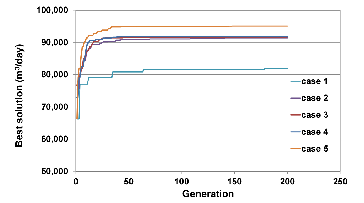
Table 4 shows the best solution generated after 200 iterations as well as the central processing unit (CPU) time for the simulation of five cases. The conventional GA yielded the least optimal solution (81,957 m3/day), while the maximum pumping rate of approximately 95,059 m3/day was obtained in Case 5. As each operator improved individually, the value of the best solution exceeded those of the previous cases. This means that the adopted operators (real number encoding, multipoint crossover, dynamic penalty function, and cluster exchange) improved the GA. Real number encoding and cluster exchange particularly contributed to the improvement. However, real number encoding increased the computational cost in comparison with binary encoding. This is interesting as the binary string is longer than the real number string used in this study. Case 1 contained 84 strings for binary encoding, whereas the individuals of Case 2 used only six strings for real encoding. Compared with Cases 3 and 4, the computing times of Cases 1 and 2 were shorter. However, the reduction of computational effort owing to the dynamic penalty function was unclear.
Table 4.
Best solutions and computing efforts for five cases
| Best solution (m3/day) | CPU time (sec) | |
| Case 1 | 81,957 | 41.37 |
| Case 2 | 91,428 | 46.22 |
| Case 3 | 91,703 | 49.83 |
| Case 4 | 91,800 | 47.78 |
| Case 5 | 95,059 | 48.28 |
Fig. 5 compares the changes in the best solutions with each iteration for the five cases. Real-number-encoded cases converged more quickly than binary-encoded cases. In particular, the cluster operator required fewer generations to converge than did the other cases.
Conclusion
Various factors can induce spatio-temporal changes in Korean aquifers. Seasonal changes greatly influence groundwater resources, and various solutions should be explored to carefully manage groundwater use during periods of drought. This study increased the rate of manageable groundwater extraction. by improving the GA technique developed in previous studies. Changing the structure of the GA significantly improved the solution for well pumping. In particular, “real number encoding” and “cluster exchange” yielded the most significant improvements. At such as facility cultivation sites, pumping wells with small-capacity motors are typically densely clustered, and the proposed method can optimize their response to drought and water shortage as the non-decision variables of clusters can be exchanged. In the future, we will investigate the application of this technique to actual sites. In addition to the possibility of this technique increasing groundwater development, it could also be applied to establish efficient strategies for the artificial regeneration of aquifers.
Appendix
Pseudo-code of algorithm:
Set parameter values
Generate random initial solution for Qi with population ps
For gen = 1 to generation
For i = to ps
For i = 1: number of pumps
Calculated head with well pumping equation
End
End
If (hi,ps <0)
Evaluate fitness (F) =
end
If (F > best solution thus far)
best solution = F
end
Record best solution with iteration number
for 1:ps/2
If (rand <pc)
Tournament and select parent
Generate binary_mask % the array size is the same as the well number
Crossover according to binary_mask array with probability, pc
End
If (rand< pm)
Mutation 1: gene swap in offspring 1 with probability, pm
gene swap in offspring 2 with probability, pm
Mutation 2: put real value in one gene of offspring 1 with probability, pm
put real value in one gene of offspring 2 with probability, pm
End
End
If (rand <pc) % cluster exchange
For i = 1 to well_number/2
x(i) = x(well_number/2+1-i)
End
End
End
