Introduction

Morphological characteristics of rock discontinuities directly influence the strength and deformation characteristics of rock. Due to the complex formation conditions and occurrence environments of discontinuities in natural rock,morphologies of these discontinuities are characterized by waviness, complexity, poor regularity, and randomness. Therefore, how to accurately measure and characterize morphological characteristics of discontinuities has always been a difficult and hot point in the mechanics research of rock discontinuities.

With regard to characterization methods of morphologies of rock discontinuities, natural discontinuities are rough and have asperities of different dip angles and heights. The geometrical elements of these discontinuities include the strike, dip (dip direction and angle), continuity (along the strike and dip directions and determined based on the cutting degree), roughness and waviness (amplitude and length). Barton first proposed the concept of the joint roughness coefficient (JRC) in 1973 (Barton, 1973) and established the relationship of normal stress σn, peak shear strength τ, internal friction angle ϕb, and compressive strength σc with the joint roughness. Then in 1977, Barton provided ten standard profile curves using the standard profile reference method (Barton and Choubey, 1977). Tse and Cruden (1979) took the lead to determine the JRC value using the statistical parameter-based method. They used the slope root mean square (RMS) Z2 and the structure function (SF) to estimate the JRC value and provided the fitting relationship of the two with the JRC value. The concept of slope RMS Z2 was proposed by Myers (1962) and the parameter can be used for quantitative description of the roughness of rock discontinuities. On this basis, Belem et al. (2000) and Zhang et al. (2009) came up with the expression for the three-dimensional (3D) slope RMS. Zhang et al. (2014) provided improvement based on the two-dimensional (2D) slope RMS Z2 and considered anisotropy of roughness of discontinuities, thus providing the improved slope RMS Z2'. The SF is another parameter proposed by Saylers and Thomas (1977) for describing roughness of discontinuities. Chen et al. (2021) found that among various statistical parameters, the slope RMS Z2 and the SF are of the highest correlation with the JRC, and they proposed a general method for determining the JRC with combined parameters of any sampling interval. The waviness angle θ is a commonly used index for describing morphological characteristics and studying mechanical properties of discontinuities, whose measurement and calculation methods have been studied by Patton (1966), Guo (1982), Turk and Dearman (1985), and Belem et al. (2000). Initially, the waviness angle θ was only applicable to description of the dip angle of a single asperity on discontinuities. Then, numerous scholars have proposed the angle for evaluating the overall waviness of discontinuities, that is, the generalized waviness angle.

For the evaluation of morphological characteristics of discontinuities, scholars at home and abroad have never stopped their efforts in researching new methods and parameters. Due to the complexity and randomness of morphological characteristics of discontinuities in natural rock, it still has not been able to determine parameters that can optimally describe surface morphologies of discontinuities. Existing research not only points out the non-reasonability of describing joint morphologies with a single parameter (Liu and Sterling, 1994; Xie et al., 1997), but also considers that the description results of morphological characteristics of discontinuities with multiple parameters also differ from the real conditions. For examples, Bahat (1991) evaluated morphological characteristics of discontinuities with 14 parameters that almost cover all aspects of these morphological characteristics. This shows that it is challenging to accurately describe the morphological characteristics of rock discontinuities. More importantly, one of the main purposes for characterizing morphological characteristics of discontinuities is to explore influences of different morphological characteristics on shear properties of discontinuities. However, existing research hardly provides the description method for morphological characteristics of discontinuities by combining with shear behaviors of discontinuities. Grasselli et al. (2002) proposed a method for describing morphological characteristics of discontinuities using the statistical function relationship between the effective shear angle of infinitesimal elements on discontinuities and the corresponding contact area. Despite this, parameters in the method do not have definite physical meanings. Combining the directivity of shear behaviors of discontinuities, Song et al. (2017) put forward the 3D shear coefficient SC3D to describe discontinuities and proved that the parameter can well reflect the anisotropy of morphological characteristics of discontinuities through specific examples.

Discontinuities in natural red sandstone were taken as research objects to perform the 3D morphological scanning test and obtain morphological data of discontinuities. In addition, the wavelet transform was adopted to separate waviness and roughness from morphological characteristics. In this way, the index and evaluation method for 3D morphological characteristics of rock discontinuities considering the shear direction were proposed.

Acquisition of 3D Morphologies of Rock Discontinuities

Sample Preparation

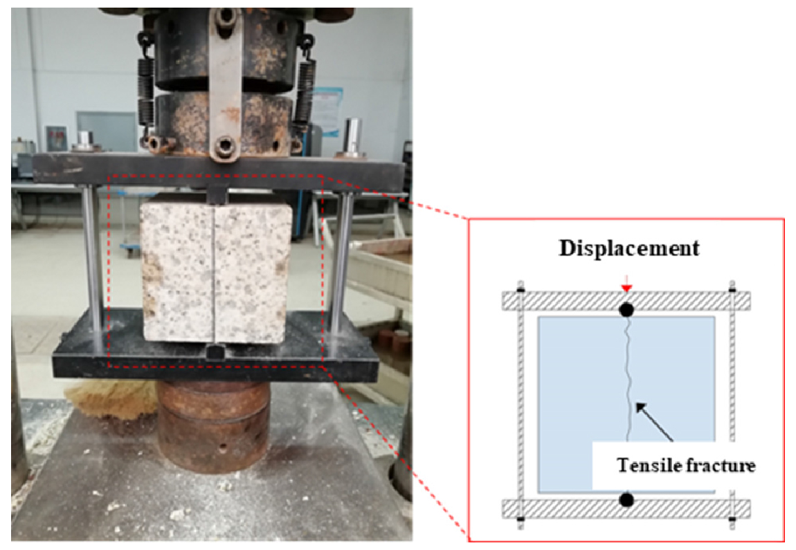
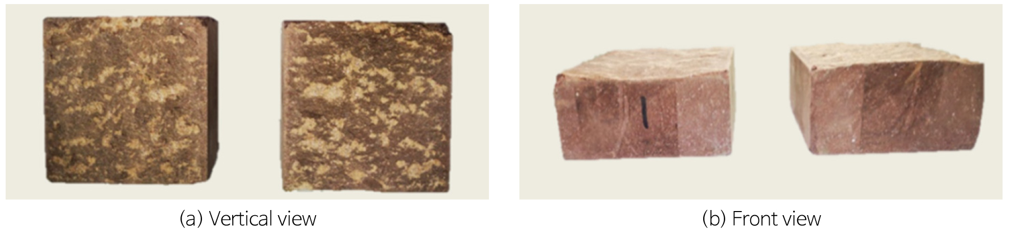
Natural red sandstone blocks collected in the field were used, which were cut into cubic samples measuring 100 mm × 100 mm × 100 mm (length × width × height) with a specific rock cutting tool. Then, the splitting test (Fig. 1) was conducted to split the above samples at the central line, thus obtaining samples of discontinuities of natural red sandstone (Fig. 2). The samples were labeled as No. 1~8. The surface of the natural rock was rough and contained asperities of different dip angles and heights. The anisotropy and diversity of the discontinuities were ignored to some extent.

Fig. 1.

Splitting test.

Fig. 2.

Sample of rock discontinuities.

Test Equipment

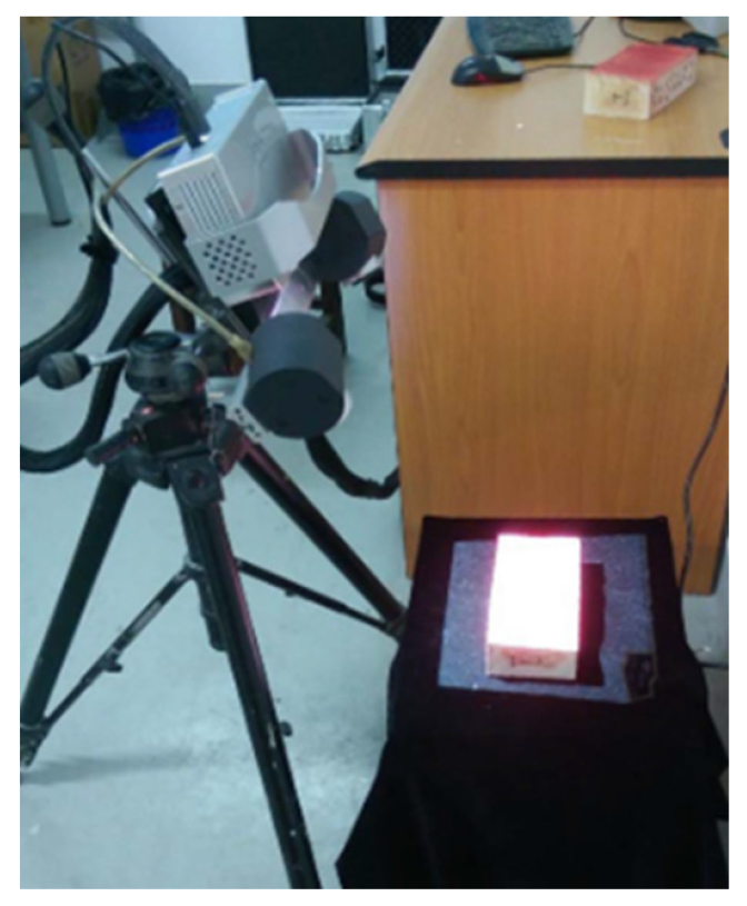
The TJXW-3D 3D surface profilometer (Fig. 3) for rock developed by the research team led by professor Xia in Tongji University was used to acquire data about surface morphologies of samples of discontinuities. The instrument is compared of three parts: a scanner, a frame, and a high-end computer. Therein, as an optical measurement structure and the core component of the instrument, the scanner consists of two high-resolution CCD industrial cameras, two industrial lenses, and a digital grating projector.

Fig. 3.

TJXW-3D 3D surface profilometer.

Test Process

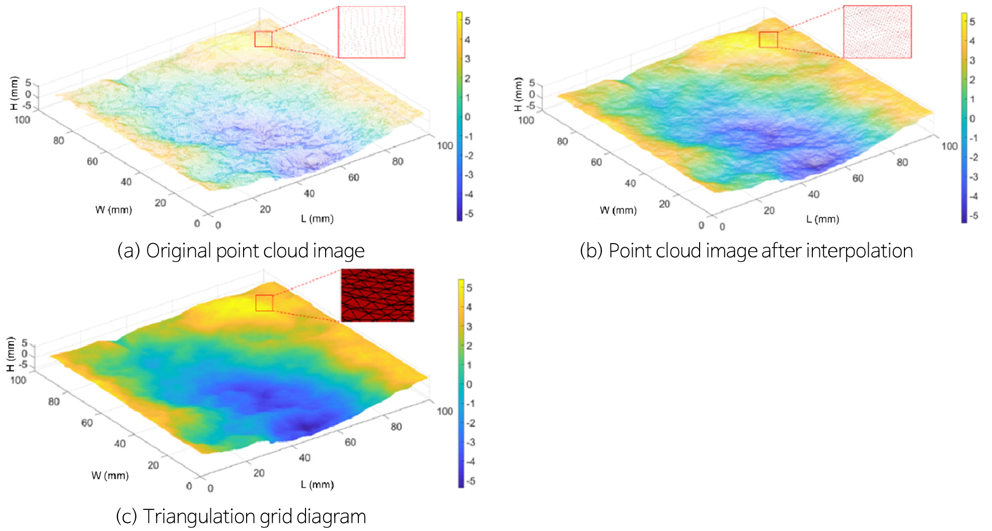
The point cloud data acquired through the 3D morphological scanning test of rock discontinuities are distributed with poor regularity, which is unconducive to subsequent data processing. Therefore, the raw data need to be interpolated to attain equally spaced 3D point cloud data of discontinuities. Tatone (2010) conducted lots of direct shear tests on jointed rock and found that the morphological data can well reflect the waviness of joints when the interval of data points is smaller than 0.55 mm and are enough to capture detail features of local roughness of joint surfaces. The characterization parameter for roughness calculated in this way can be used to study shear properties of jointed rock.

By comprehensively considering the sample size of discontinuities, calculation accuracy and efficiency, the data interval used in the research was 0.2 mm. The original data were subjected to interpolation based on the interpolation algorithm in the MATLAB with 500 sampling points in both the length and width directions of discontinuities and totally 250,000 data points. The 3D morphological data of rock discontinuities were still processed and presented as points, which failed to intuitively reproduce the real morphologies of discontinuities and the points should be further transformed to faces. Delaunay triangulation is able to connect spatial points into triangles that are characterized by the highest proximity, uniqueness, optimality, highest regularity, and locality, so it is the most widely used triangulation method in the practice. Fig. 4 illustrates the interpolation and triangulation results of point cloud data about discontinuities of jointed rock.

Fig. 4.

Interpolation and triangulation results for point cloud data (taking the discontinuity in specimen 1 as an example) .

Separation of Waviness and Roughness from 3D Morphologies of Rock Discontinuities

Basic Principles of Wavelet Transform

At present, wavelet transform has been widely used in many fields including signal processing, seismic prospecting, fluid turbulence, and image processing. The morphologies of discontinuities of natural jointed rock in the research not only produce all kinds of frequency signals but also include local characteristics such as asperities almost without any period or frequency characteristics. The morphological data can be refined and analyzed at multiple scales and local features or specific frequency can be extracted and reproduced in the space domain by using wavelet transform, thus realizing multi-scale decomposition and synthesis of morphologies.

Discontinuities of natural rock mainly contain relatively large asperities that describe the fluctuation trend of discontinuities and little ones that characterize the roughness, which can be separately described using the waviness and roughness. Previous research has demonstrated that waviness and roughness have different influence mechanisms on the shear mechanics of jointed rock, with the former corresponding to shear resistance of asperities while the latter to the friction resistance.

According to definitions of roughness and waviness as well as suggestions of the International Society for Rock Mechanics (ISRM, 1978), the low-frequency and high-amplitude f1(x,y) is used as the first-order waviness while the high-frequency and low-amplitude f2(x,y) as the second-order roughness. Then, the mathematical model for 3D morphologies of rock discontinuities can be written as

It is worth noting that the 2D decomposition of morphologies of discontinuities is performed using the one-dimensional (1D) wavelet transform; while 3D analysis uses the 2D Mallat algorithm following such a principle: row data in the 3D morphologies are first subjected to 1D wavelet transform and then the transformed data undergo the second 1D wavelet transform by columns.

where, anj and dnj are the nth calculated values of the low-pass and high-pass jth layers; hn and gn represent the low-pass and high-pass filter coefficients, respectively.

Morphological data after 2D discrete wavelet transform can be decomposed into approximate morphological components at a certain resolution (low-frequency morphologies (waviness)) and detailed morphological components in vertical, horizontal, and diagonal directions (high-frequency morphologies (roughness)).

Selection of the Optimal Wavelet Basis Function

There are various wavelet functions. As long as a function meets the admissible conditions of wavelets, it can be used as a wavelet function. The admissible condition is expressed as the formula below:

where, ψ^(ω) is the Fourier transform of ψ(t), and ψ(t)∈L2(R).

Common wavelet functions include Haar wavelet, Daubechies wavelet system, Symlet wavelet system, Coiflet wavelet system, and Biorthogonal wavelet system. When selecting wavelet functions, the orthogonality, symmetry, regularity, short support, and high-order vanishing moments should be met at the same time as far as possible. However, all of the common wavelet functions cannot simultaneously meet the above requirements, which therefore should be traded off. In addition, because selection of wavelet functions still lacks a definite standard, the wavelet decomposition is highly uncertain. That is to say, morphological separation of rock discontinuities yields different results when using different wavelet functions.

Therefore, orthogonal wavelet functions are given priority in the selection to avoid loss of original morphological information during wavelet transform. The preliminarily selected wavelets include Daubechies, Symlet, and Coiflet wavelet systems. Subsequently, the optimal wavelet function is determined by comparing difference between the reconstructed data of 3D morphologies by different wavelet basis functions after the same times of decomposition and the original data. The discontinuities used in the research measure 100 mm × 100 mm (length × width) with 250,000 sampling points after interpolation, that is, there are separately 500 sampling points on both the length and width directions of discontinuities, so N = 500. The maximum theoretical scale of wavelet transform is jmax=[log2N]=8, which means that the 3D morphological data undergo eight times of decomposition at most. In summary, 21 wavelet basis functions are used to perform eight times of decomposition and reconstruction of any 3D morphologies of rock discontinuities to attain the reconstruction error. Table 1 lists the wavelet reconstruction errors for 3D morphologies of rock discontinuities using different wavelet basis functions. As shown in the table, the morphologies decomposed and then reconstructed with the wavelet basis function sym5 exhibit the smallest error with the original morphologies, so wavelet basis sym5 is selected to separate morphologies of discontinuities of jointed rock. The main properties of sym5 are displayed in Table 2.

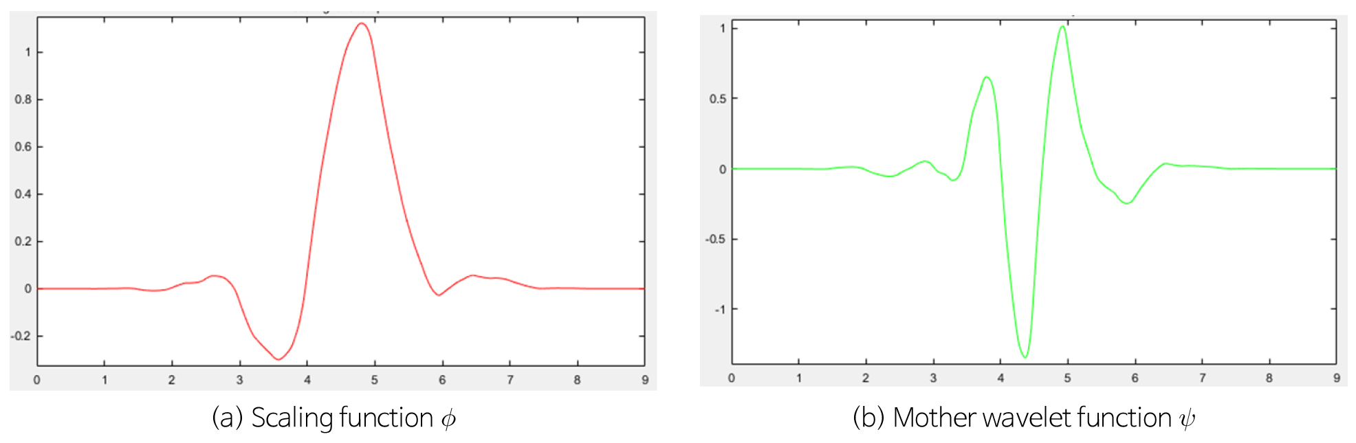
Symlets wavelet is a compactly supported orthogonal wavelet constructed by Daubechies without a specific analytic expression. Fig. 5 shows the father wavelet function ϕ (scaling function) and mother wavelet function ψ of sym5 wavelet. The sym5 wavelet basis function is attained through scaling and translation of the father and mother wavelet functions. In the process, the scaling multiple is an order of 2 and the translation amplitude is related to the scaling degree. Then, the form of wavelet expansion for discrete signals with a sampling size N is expressed as follows:

where, k and j represent the translation amplitude of the function and the number of decomposed layers, respectively; Tϕ(0,0) and Tψ(j,k) separately denote the approximation coefficient and the refinement coefficient.

Fig. 5.

The sym5 wavelet.

Selection of the Optimal Number of Decomposed Layers

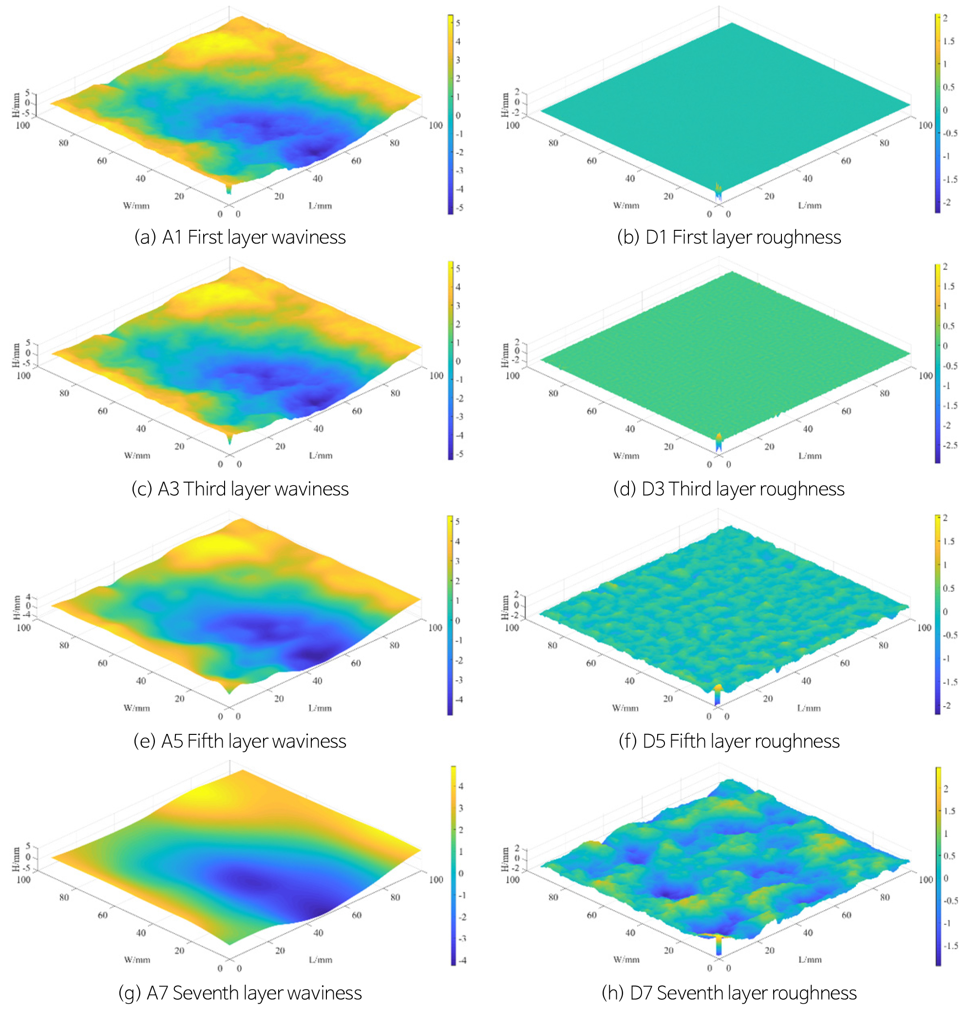
Figure 6 shows the decomposition results of 3D morphologies of rock discontinuities by using the wavelet basis function sym5 (taking the No. 1 discontinuity as an example). The morphologies were decomposed for eight times at the maximum theoretical scale of wavelet transform. A1~A8 represent the approximate signals decomposed with the low-pass filter, that is, the first-order waviness; D1~D8 denote the high-frequency detail signals, namely, the second-order roughness. It is worth noting that the high-frequency detail components obtained through wavelet transform actually include three parts in the vertical, horizontal, and diagonal directions. The signals acquired by subtracting low-frequency data from the original morphologies are directly used as the second-order roughness, for the sake of simplification and more clear results. The 3D morphologies of rock discontinuities are A1+D1 = A2+D2 = A3+D3 = A4+D4 = A5+D5 = A6+D6 = A7+ D7 = A8+D8.

As shown in Fig. 6, most waviness information in the original morphologies of discontinuities has been lost in the approximate signal A of these morphologies with the increasing number of decomposed layers; correspondingly, obvious undulating morphologies occur to the high-frequency detail signal D which shows the low-frequency phenomenon. The result is apparently contrary to the initial decomposition purpose, so it needs to determine the optimal number of decomposed layers by wavelet transform.

Fig. 6.

Three-dimensional topography decomposition of rock discontinuities (unit: mm).

The method for determining the optimal number of wavelet-decomposed layers proposed by Zou et al. (2015) and Wang et al. (2016) was used. The optimal number is determined according to the variance of the first-order waviness. When decomposing to a certain layer, the variance of the first-order waviness changes dramatically. In the case, the number of decomposed layers before the current decomposition is taken as the optimal number of wavelet-decomposed layers for 3D morphologies of discontinuities. The method is based on the principle that the main waviness characteristics of original morphologies can be maintained when the variance of the first-order waviness is approximated to that of original morphologies. Fig. 7 shows variances of the first-order waviness of rock discontinuities under different numbers of decomposed layers. In the figure, the layer 0 represents the variance of original morphologies. It can be seen from the figure that the variance of the first-order waviness of rock discontinuities decreases significantly when the number of decomposed layers reaches 6. Therefore, the optimal number of decomposed layers is 5.

Fig. 7.

Relationship between first-order waviness variance and decomposition layers.

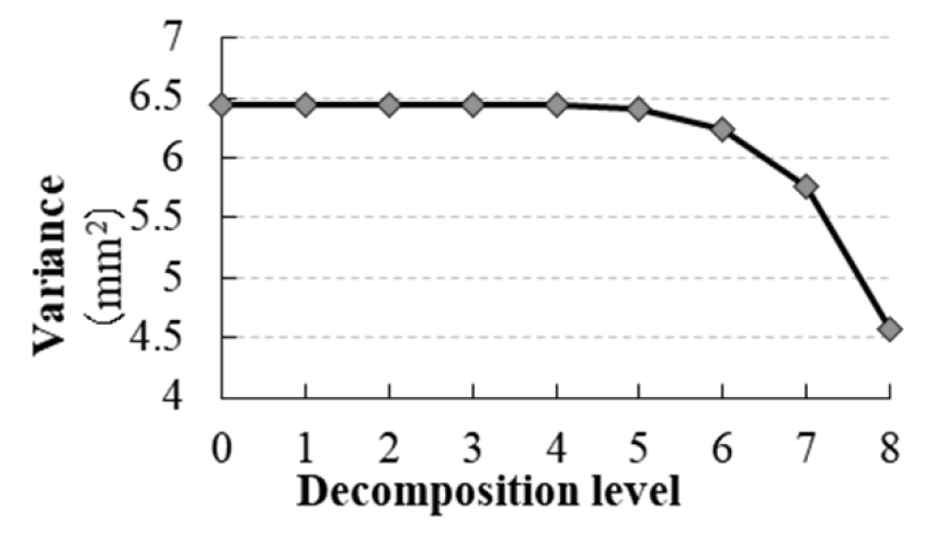
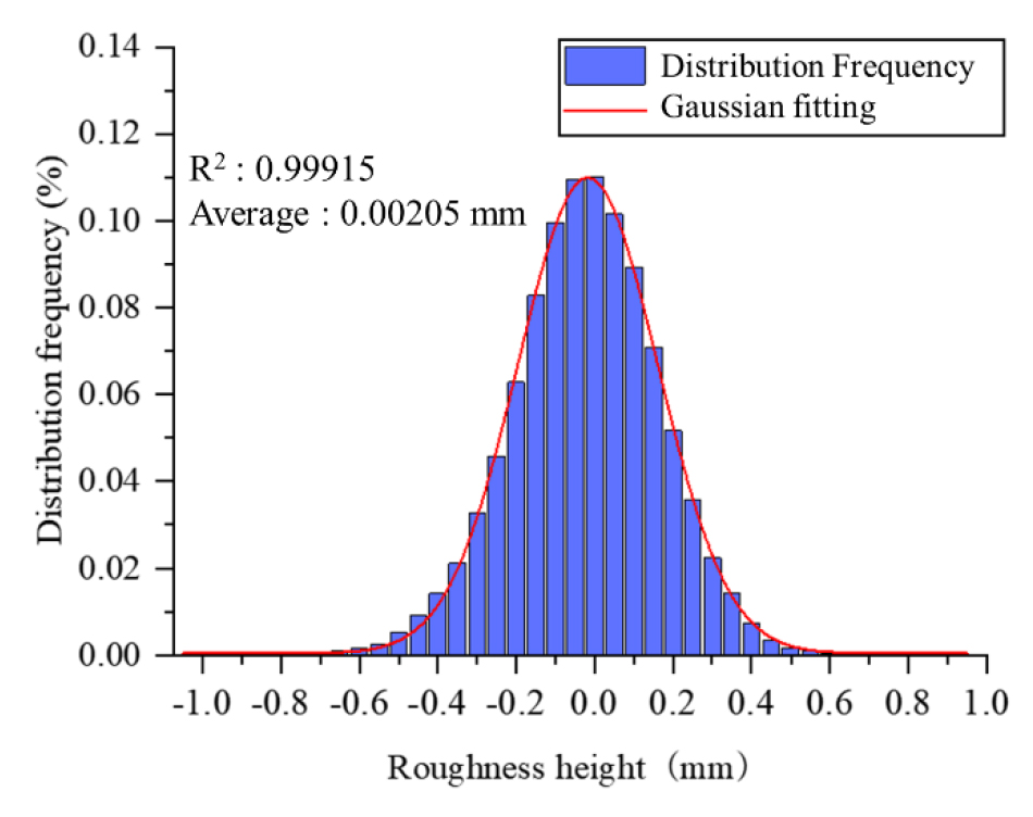
Figure 8 illustrates the distribution frequency histogram of the waviness height when the 3D morphologies of rock discontinuities are decomposed to the fifth layer. The average waviness height is 0.00205 mm (approximating to 0) when fitting with the Gauss function. The correlation coefficient R^2 is 0.999, which is larger than 0.99, indicating that the waviness follows the Gaussian normal distribution after separation. The conclusion agrees with the research results of Zou et al. (2015) and Wang et al. (2016), which indirectly proves the reasonability of the decomposition results in the research.

Fig. 8.

Distribution frequency histogram for waviness height.

Indexes for 3D Morphological Characteristics of Rock Discontinuities considering the Shear Direction

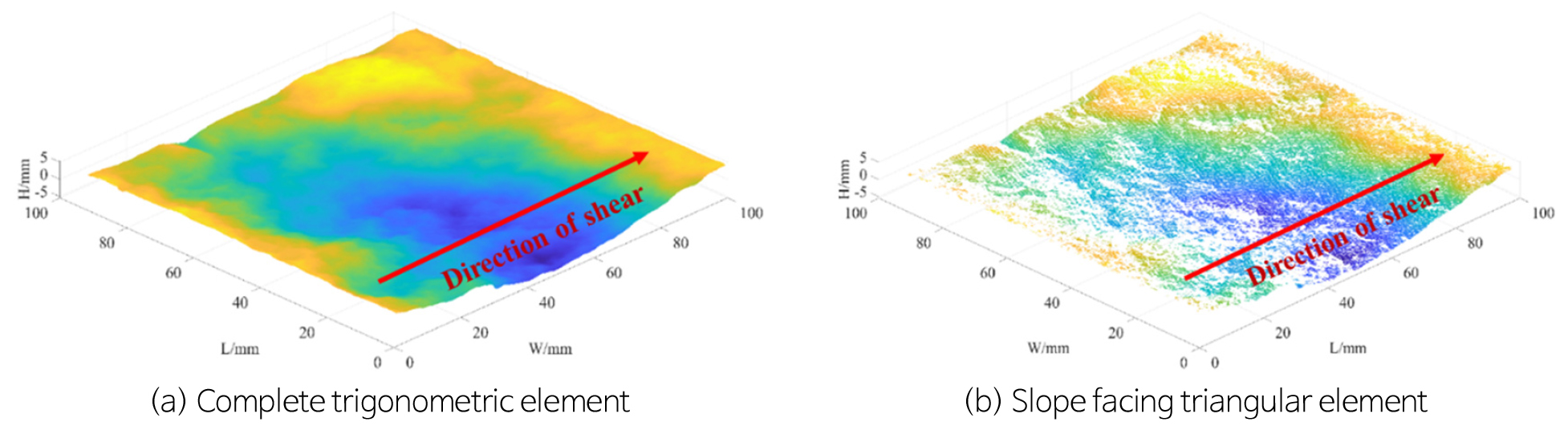
Some scholars have found through the direct shear tests of rock discontinuities that the upper and lower discontinuities are only partially contacted in the shear process and they are only in contact on the slope facing the shear direction. Therefore, triangular infinitesimal elements on discontinuities that face the shear direction are screened at first before evaluating 3D morphological characteristics of rock discontinuities, as shown in Fig. 9.

Fig. 9.

Triangulation element screening for shear direction.

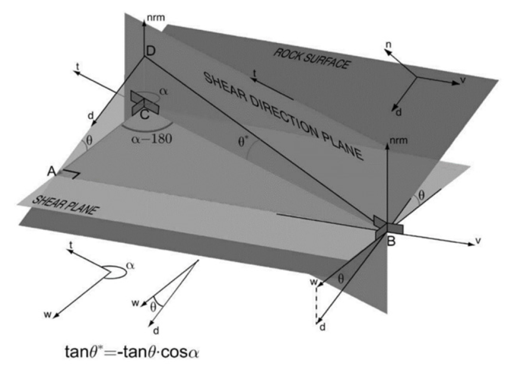
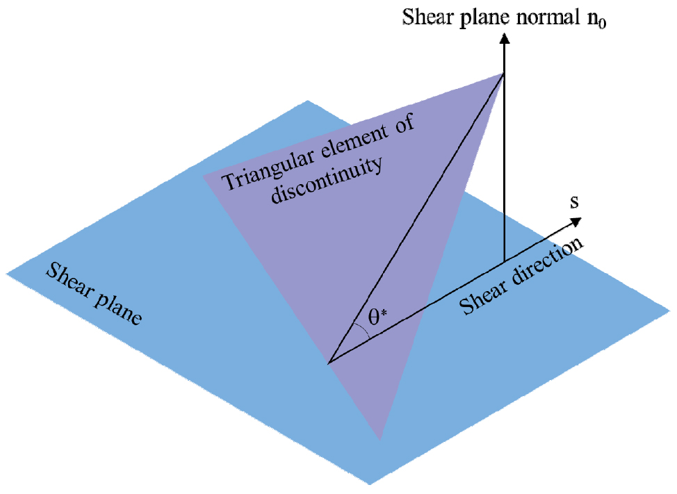
For screened data, the relationship between the apparent dip angle θ* of triangular infinitesimal elements and shear direction is clearly defined based on the geometric definition of the apparent dip angle θ* considering shear direction proposed by Grasselli et al. (2002), as shown in Fig. 10 and Fig. 11.

Fig. 10.

Geometric definition of apparent dip angle θ* considering shear direction.

Fig. 11.

Schematic diagram of the apparent dip angle θ* considering the shear direction.

Based on the effective shear angle θ* of triangular infinitesimal elements on the slope-facing plane, the calculation formula for the slope RMS Z2+ of discontinuities considering the shear direction is proposed:

where, θi* represents the effective shear angle of the ith triangular infinitesimal element and n denotes the overall effective shear angle.

Formula (7) is only related to the effective shear angle of discontinuities. After obtaining the point cloud data of discontinuities through the 3D morphological scanning test, the refined effective shear angle can be calculated, which can describe characteristics of triangular faces of each triangular infinitesimal element on the discontinuity. The slope RMS Z2+ calculated can accurately describe morphological characteristics of the whole discontinuity. It is calculated rapidly and can be used as an effective parameter for describing morphological characteristics of discontinuities.

The overall slope RMS Z2+ before separation and slope RMSs Z2w+ and Z2r+separately of waviness and roughness are calculated according to Formula (7), and the results are listed in Table 3. It can be seen from the table that the overall RMS Z2+ of each discontinuity is between the slope RMSs Z2w+ and Z2r+ separately of waviness and roughness, and Z2r+ is slightly larger than Z2w+. Comparison of upper and lower discontinuities reveals that the slope RMS Z2r+ of roughness has a larger mean deviation than the slope RMS Z2w+ of waviness. That is to say, the slope RMSs of waviness of upper and lower discontinuities remain basically consistent while those of roughness have certain difference, which results from uncertainty of surface morphologies of natural discontinuities. Therefore, the mean value of the overall slope RMS Z2+ and slope RMSs Z2w+ and Z2r+ separately of waviness and roughness is used to characterize the 3D morphological characteristics of rock discontinuities.

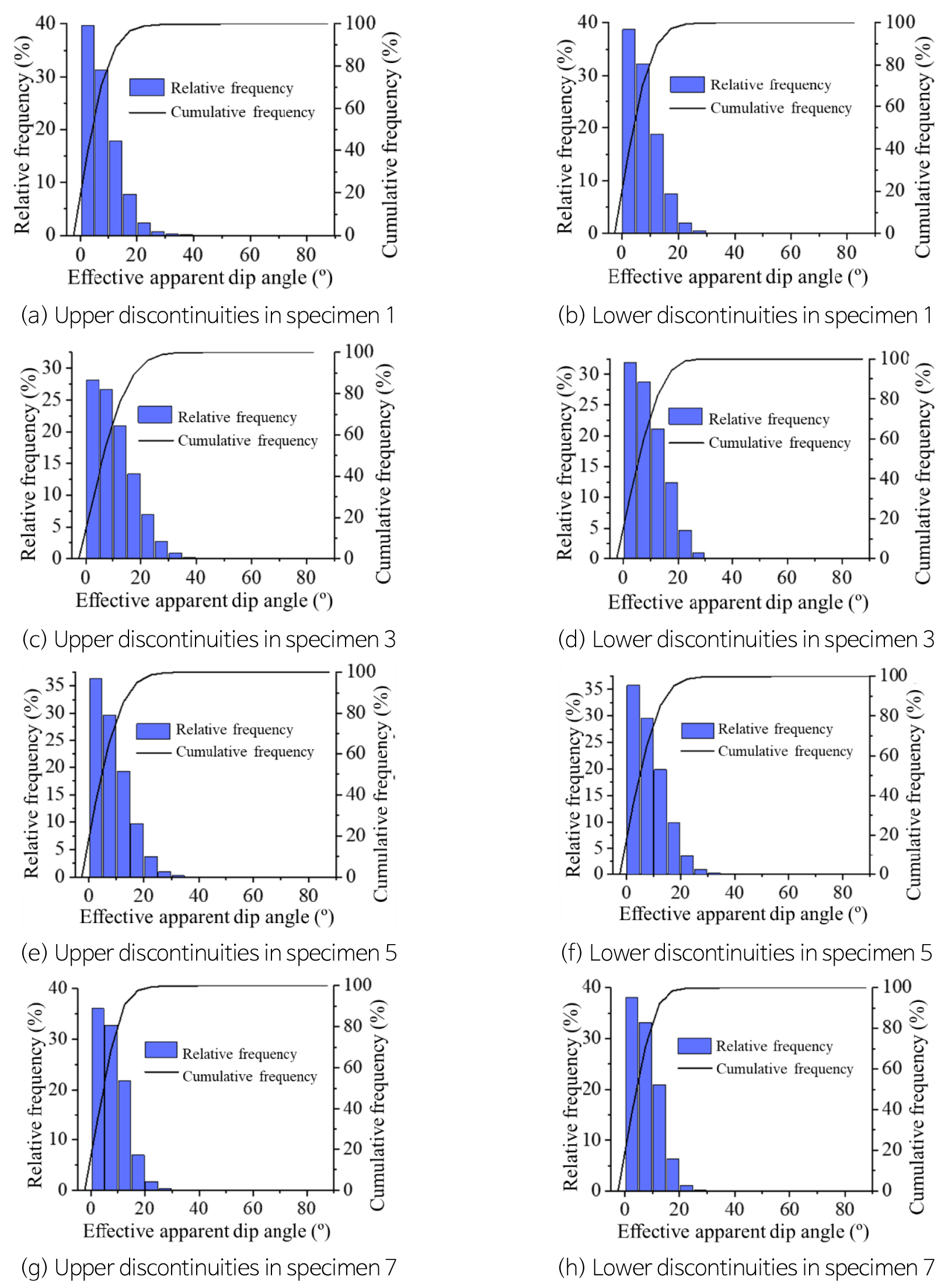
Moreover, Fig. 12 illustrates the statistical results for distribution of the overall effective apparent dip Angle of discontinuity samples (taking the No. 1, 3, 5, and 7 samples as examples) to describe 3D morphological characteristics of discontinuities as comprehensively as possible. As shown in the figure, the effective apparent dip angle of discontinuities is generally in the range of 0~10°, and the cumulative frequency of the effective apparent dip angle of each discontinuity in the range exceeds 80%. The effective apparent dip angle is mainly shown as low-angle friction; while the rest large effective apparent dip angle serves as teeth to resist slip and shear of discontinuities and is shown as high-angle waviness in discontinuities.

Fig. 12.

Distribution of effective apparent dip angle for discontinuities.

Conclusions

The accurate measurement and quantitative evaluation of 3D morphological characteristics of discontinuities in natural rock are the basis for studying mechanical properties of discontinuities. The research collected and prepared samples of discontinuities in natural rock, conducted 3D morphological scanning test of discontinuities, and evaluated 3D morphological characteristics of discontinuities based on the scanning data. The obtained conclusions are listed as follows:

(1) The 3D morphologies of discontinuities in natural rock can be separated into waviness and roughness using the sym5 wavelet basis function. The two separately characterize the shear resistance and friction resistance of discontinuities.

(2) The calculation method for the slope RMS of 3D morphologies of discontinuities considering the shear direction was proposed based on the concept of effective shear angle. Combining with the morphology separation results, concepts of slope RMSs of waviness and roughness were put forward.

(3) The overall slope RMS is between the slope RMSs of waviness and roughness. For a same group of discontinuities, the slope RMSs of waviness of the upper and lower discontinuities basically remain consistent, while those of roughness differ greatly. Finally, the mean value of the above three slope RMSs was determined as the evaluation index for 3D morphological characteristics of discontinuities.