Introduction

Recently, research using hyperspectral images has been actively conducted in various fields. With the miniaturization of hyperspectral sensors, mounting drones and obtaining high spectral resolution and continuous band wavelength and studying specific spectral characteristics for targets has become possible.

Hyperspectral images consist of more than 200 consecutive bands for spectral wavelength regions. Furthermore, the spectroscopic information of the target is expressed more similarly, enabling more detailed analysis compared to conventional multispectral images (van der Meer, 2003; Kim et al., 2010; Rasti et al., 2018). The complete properties of the surface material can be acquired from band to band, it is useful to analyze indicator properties that are difficult to detect using multispectral images (Goetz, 1991; Shaw and Burke, 2003; Heo et al., 2010; Lowe et al., 2017). Therefore, various applications are being explored in agriculture, environment, and biology as well as in the geological fields (Gowen et al., 2007; Brewer et al., 2008; Akbari et al., 2010).

Previous studies include the study of hydrothermal alteration mapping using Airborne Visible Infrared Imaging Spectrometer (AVIRIS) hyperspectral data, the analysis and classification of metamorphic rocks using reflectance spectra of hyperspectral data and the study of compositional mineral distribution using thermal infrared hyperspectral scanners (Crósta et al., 1998; Longhi et al., 2001; Kirkland et al., 2002). Furthermore, image classification and classification of urban areas were performed using high-resolution aerial hyperspectral images and used for urban cladding classification and soil contamination and evaluation (Herold et al., 2003; Mars and Crowley, 2003; Benediktsson et al., 2005; Choe et al., 2008). Moreover, a study was conducted to develop a rock characteristic cross sectional schematic of contact metamorphic aureole using spectroscopic analysis method, and a study regarding spectroscopic information analysis of unclear geological outcrop was also published (van der Meer and Kato, 2002; van der Meer, 2003).

Recently, studies regarding the mapping of ore with ultramafic rocks as country rocks using hyperspectral images and automatic mapping of rocks using hyperspectral data have been published (Rogge et al., 2014; Kumar et al., 2020). Hyperspectral images were used for field investigation of cladding degree and target detection on the surface of the earth (Manolakis and Shaw, 2002; Mhanolakis et al., 2003). In addition, studies have been conducted to analyze the composition of topsoil in the soil field, and soil composition analysis via visible and near infrared ray is efficient and non-destructive, which is used in various ways (Srodon et al., 2001; Brown et al., 2006; Nocita et al., 2013). A study regarding the analysis of geological and minerals using hyperspectral equipment was also conducted (Boesche et al., 2015; Koerting et al., 2015; Rogass et al., 2017; Krupnik and Khan, 2019, 2020). In particular, it is being used to investigate and map mineral resources and spectral libraries via image analysis (Thompson et al., 2013; Laakso et al., 2015; Feng et al., 2018; Graham et al., 2018; Chattoraj et al., 2020).

However, most of the geological and rock detection studies were conducted in specific areas on rocks using ground-based hyperspectral images, possibly owing to the difficulty of obtaining hyperspectral imaging data for large areas. In addition, because existing spectral sensors require considerable weight and storage space, only point-by-point analysis is possible and monitoring large areas is challenging.

Most rocks have different conditions and physicochemical properties, and their characteristics of absorbing and reflecting light are different therefore, the distribution range and scale of rocks can be confirmed using rock-specific spectroscopic information. Thus, this work is a fundamental study of geological and rock detection using hyperspectral images. The aim of this study is to perform drone-based hyperspectral imaging on various kinds of small rock samples and to compare and classify rocks by interpreting the obtained information. Thus, hyperspectral imaging was performed on ten rocks and the peak data value and reflectance of rocks were compared. Moreover, the applicability of each rock sample was evaluated via comparison and analysis.

Materials and Methods

Method

Classifying rocks is the most basic process to be conducted for geological research. Information regarding geological and rocks distributed in the area is also essential at actual sites, such as construction and building construction. However, areas that are difficult to access, such as hillsides and cliffs, cannot be directly investigated. Geological and rock information can be obtained using the geological maps published in the past, but detailed information is required in the field. Therefore, recently, remote exploration conducted using unmanned aerial vehicles, such as drones, has been used in areas where direct investigation is difficult.

Remote exploration can collect information relatively easily from a wide range of areas, where hyperspectral images can obtain information from a variety of materials not visible to the naked eye. It is very similar in spectrum but can distinguish materials based on spectral bands and has the advantage of extracting accurate information. Furthermore, as drone mounting became possible, the utilization area has expanded, enabling remote exploration to the areas that are difficult to access.

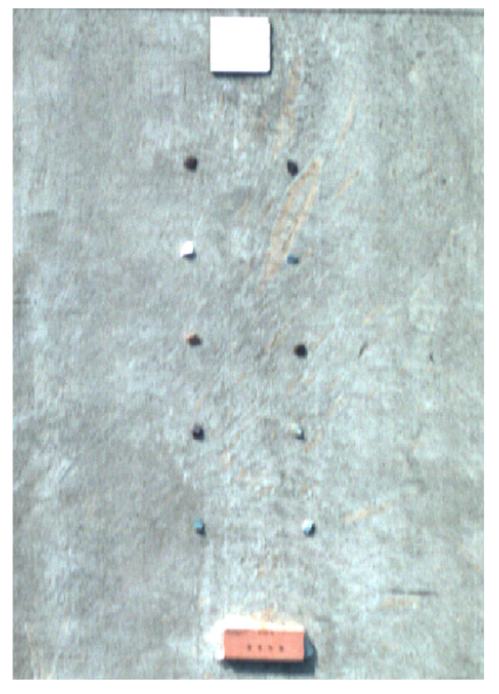
Therefore, the purpose of this study is to analyze the intrinsic information of rocks using hyperspectral sensor. The images were taken on ten rocks, and the maximum peak data value (PDV) was calculated by analyzing the values of four points for each rock (Figs. 1, 2). Data value calculated via image analysis indicates spectral radiance. The reflectance minimizes the possible error in the change of solar radiation energy using white reference with reflective characteristics of 99% or more and converts it to reflectance.

Fig. 1.

Rock samples used for hyperspectral image analysis.

Fig. 2.

Hyperspectral imaging results for ten rocks.

The acquisition of image data using drones is affected by atmospheric absorption and reflection therefore, correction is necessary. However, when spectroscopic information is obtained using a hyperspectral sensor at a low altitude in the field the atmospheric correction was not considered in this study because the radiant luminance generated in the atmosphere or energy reflected to material is rarely affected by the atmosphere.

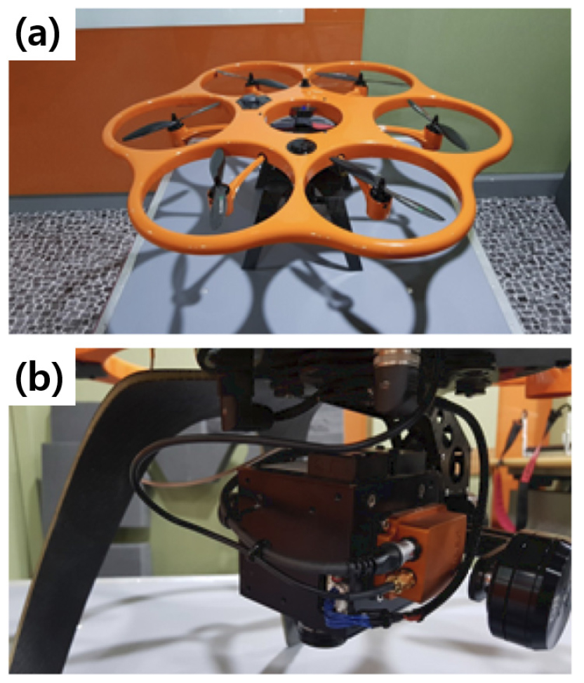
The hyperspectral sensor mounted on the drones uses Nano-Hyperspec acquired from Headwall Photonics in the United States (Table 1). It has excellent spatial and spectral resolution and high signal to noise ratio, and it can obtain high-resolution hyperspectral images of 270 bands. Moreover, the wavelength bands required by users can be divided into dozens to hundreds for collecting the spectral intensity of each band (Fig. 3a).

For the drone, the Aibot X6 (two-axis gimbal) model was used, which was provided by Aibotix in Germany. It has a loading capability of up to 3.0 kg during flight and can obtain accurate images by wirelessly controlling the GPS reception and manual control (Fig. 3b). The image analysis was performed using ENVI version 5.5 of Harris Geospatial Solutions, enabling analysis, and information extraction of multispectral materials and hyperspectral materials, various images and vector format support and the existing typical image processing basic tasks.

Fig. 3.

Drone-based hyperspectral sensor (a) Hyperspectral image sensor and (b) mounted drones.

Samples

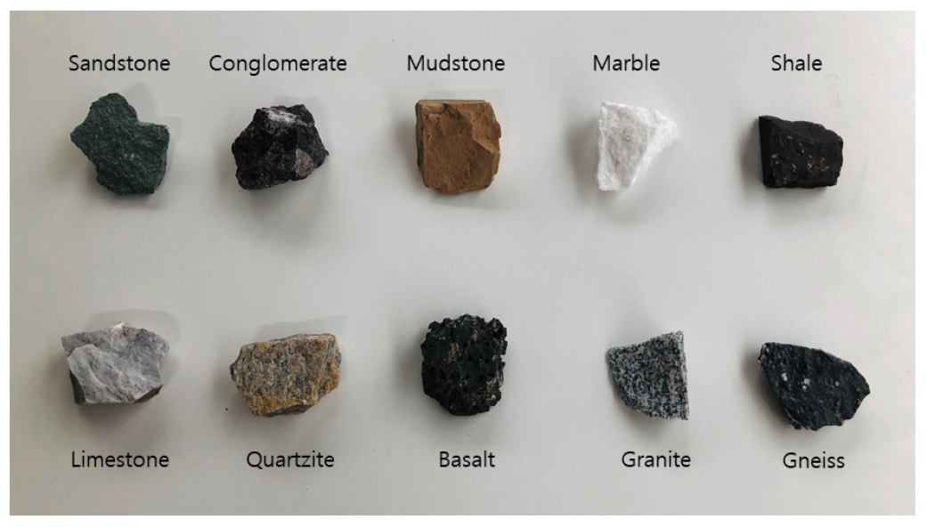
In this study, a total of ten rock samples (five sedimentary rocks, two igneous rocks, and three metamorphic rocks) were used for hyperspectral imaging. The ten rock samples can be divided into three groups sedimentary rocks including shale, mudstone, limestone, sandstone, and conglomerate samples igneous rocks including granite and basalt samples and metamorphic rocks including marble, quartzite, and gneiss samples (Fig. 1). The size of rock samples is approximately 10 m, and rocks with little particle change were selected for accurate spectroscopic information analysis.

Shale is sufficiently dark red and find-grained to prevent particles from being observed with the naked eye, and the mudstone is clear yellow in color and granular enough to prevent particles from being observed with the naked eye. Shale and mudstone are formed by the deposition of mud, but the weight of mudstone is much lighter than that of shale. Limestone is grayish white, and sandstone is pale green and find-grained that is composed of quartz, feldspar, mica and hornblend. Conglomerate is a clast and dark red matrix comprising stations of various sizes and colors.

Granite is medium-grained, with more colorless mineral content than colored minerals, and basalt is dark gray and its particles cannot be distinguished with the naked eye, and pores of various sizes are observed. Quartzite is light gray, foliation is observed, gneiss is recrystallized, a little luster is observed and the foliated surface is dark gray containing a very small amount of leucocratic.

Results and Discussion

The data value and reflectance changes of four points in each rock were compared and analyzed with ten rocks.

Comparison of Peak Data Value

Wavelength and data value for each rock point were classified into ten rocks, and analysis showed that similar patterns were shown according to red, green and blue, which are characteristics of visible ray range by rock type (Table 2, Figs. 4, 5).

Fig. 4.

Data value of each rock by wavelength.

Fig. 5.

Average data value by rock type.

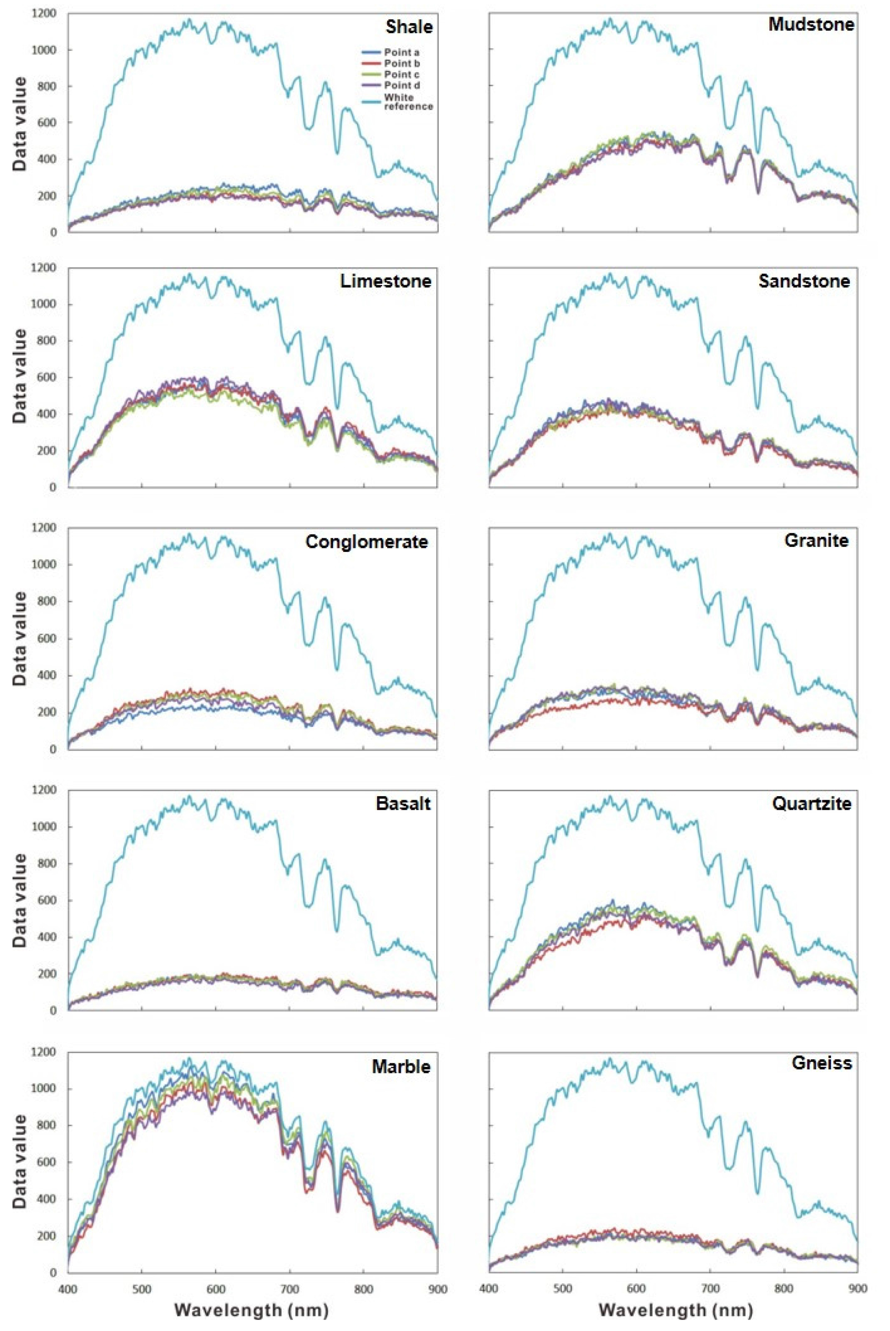
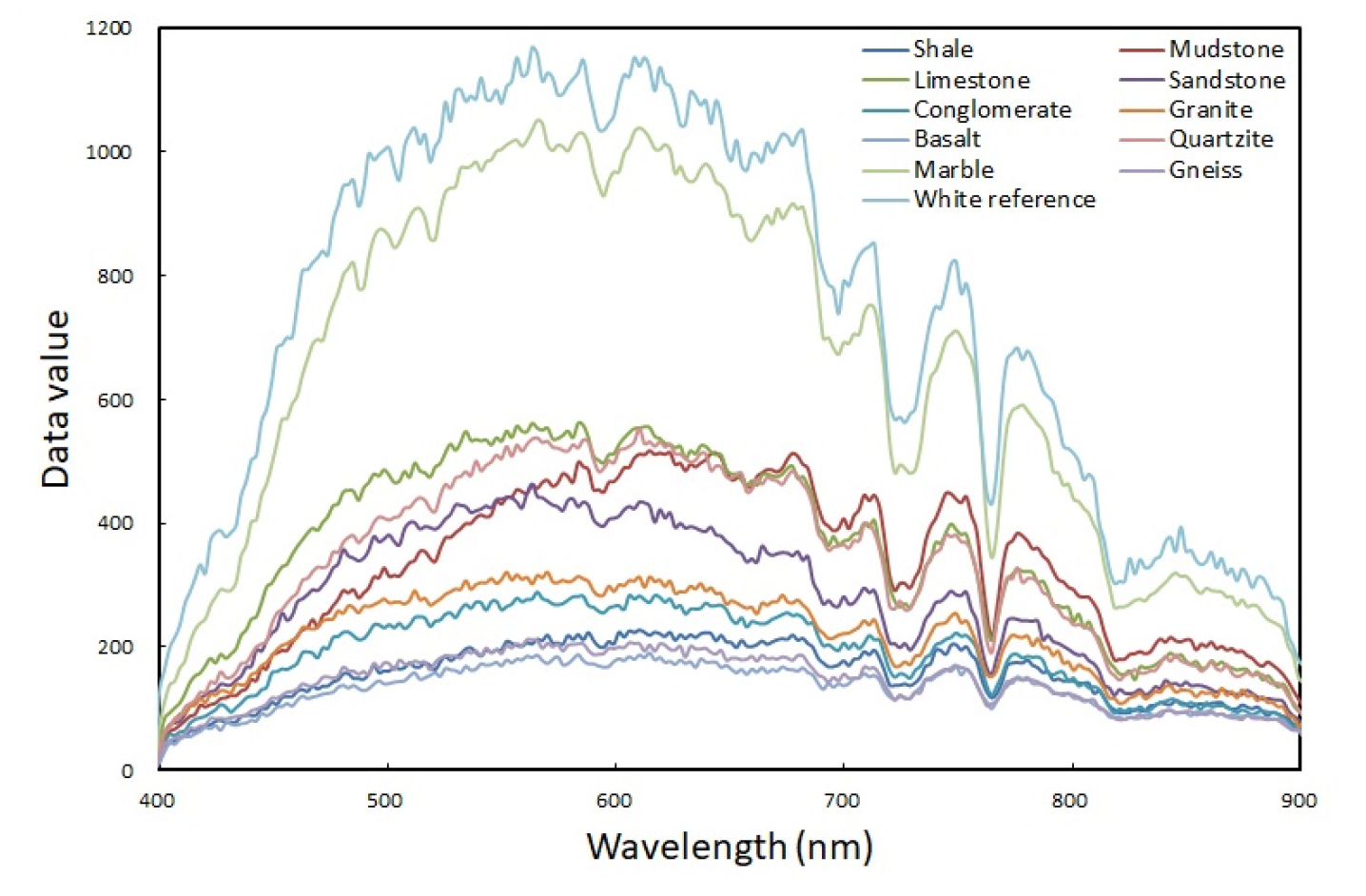
For shale, the maximum data value range for each point was shown to be 207~270, and the maximum data value was calculated to be 226.00 when the average value of consensus for each wavelength of four points was applied. Most of them had the same color, and a gentle slope appeared in the visible ray. The maximum data value range of mudstone was 505~549, and the maximum data value was 517.50 when the average value was applied to each band of four points. The maximum data value range of limestone was 540~605, and the maximum data value was 562.75 when the average value was applied to each band of four points. The maximum data value range of sandstone was 444~486, and the PDV was 463.75 when the average value was applied to each band of four points. The data values of each wavelength for four points were similar, and the PDV range was narrow. The maximum data value range of conglomerate was 245~333, and the maximum data value was 288.50 when the average value was applied to each band of four points. Similar to the case of shale, the data value range of four points was in the range of 500~700-nm wavelength.

The maximum data value range of granite was 285~358, and the maximum data value was 320.25 when the average value was applied to each band of four points. Three points showed very similar values, but one point showed a difference in data value, and it is concluded that this difference is because of the presence or absence of particles in the rock. The maximum data value range of basalt was 180~205, and the maximum data value was 189.50 when the average value was applied to each band of four points. In the graph, four points showed very similar values at most wavelengths and the slope was very gentle. The maximum data value range of quartzite was 530~603, and the maximum data value was 552.75 when the average value was applied to each band of four points. At 450~600-nm wavelengths, the data value range of the four points became wider and the gap difference appeared between points. The maximum data value range of marble was 994~1122, and the maximum data value was 1050.50 when the average value was applied to each band of four points. Among the ten rocks, data value was the highest and the band value difference of each point by wavelength was also large. The maximum data value range of gneiss was 209~244 and the maximum data value was 212.75 when the average value was applied to each band of four points. The four points showed values similar to basalt at most wavelengths, and the slope was very gentle.

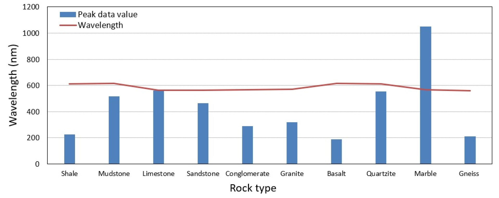
The analysis of the graph showed that the data value of marble was the highest among ten rocks and there was a difference in wavelengths between mudstone, limestone, sandstone, conglomerate, granite and quartzite however, there was a difference in data values according to the rock type. In particular, the range of wavelengths was found to be wider with increasing data value in the case of mudstone compared with other rocks. The data values as well as patterns of shale, basalt, and gneiss with low data values were similar, making it difficult to distinguish them but the difference in the data values was shown in green and red areas of 500~700 nm. Fig. 6 compares the wavelength of the PDV by rock with the PDV and shows that the wavelength of the PDV is quite similar despite a difference in the PDV, which is intrinsic information by rock.

Fig. 6.

Peak data values and wavelengths for the rock samples.

Reflectance Analysis

The reflectance of ten rocks was analyzed by comparing the data value of ten rocks with the white reference with the reflectance of 99%. The white references were set next to the rock for direct comparison with the rock data value, and the reflectance was calculated by comparing the data values (radiance) of the region (each rock region) with the standard white plates as shown in Eq. (1).

where, Vtarget denotes the data value of target and Vreference denotes the data value of reference (white reference).

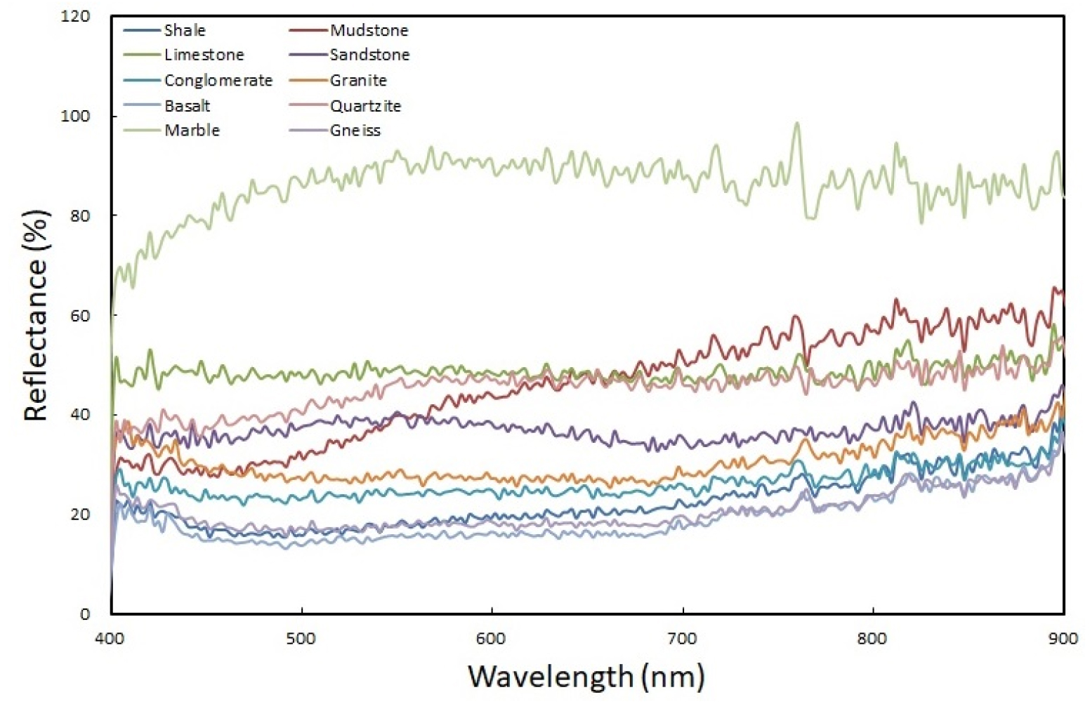
Fig. 7 is a graph showing the reflectance of four points analyzed within each rock by ten rocks, and Fig. 8 is a graph showing the average reflectance of each rock. The reflectance of the rocks was generally varied by rock in the visible ray wavelength range of 400~700 nm, and the near infrared ray range of 700 nm or more showed a gradual increase in all ten rocks.

Fig. 7.

Reflectance graph for each rock by wavelength.

Fig. 8.

Comparison graph of reflectance by rock type.

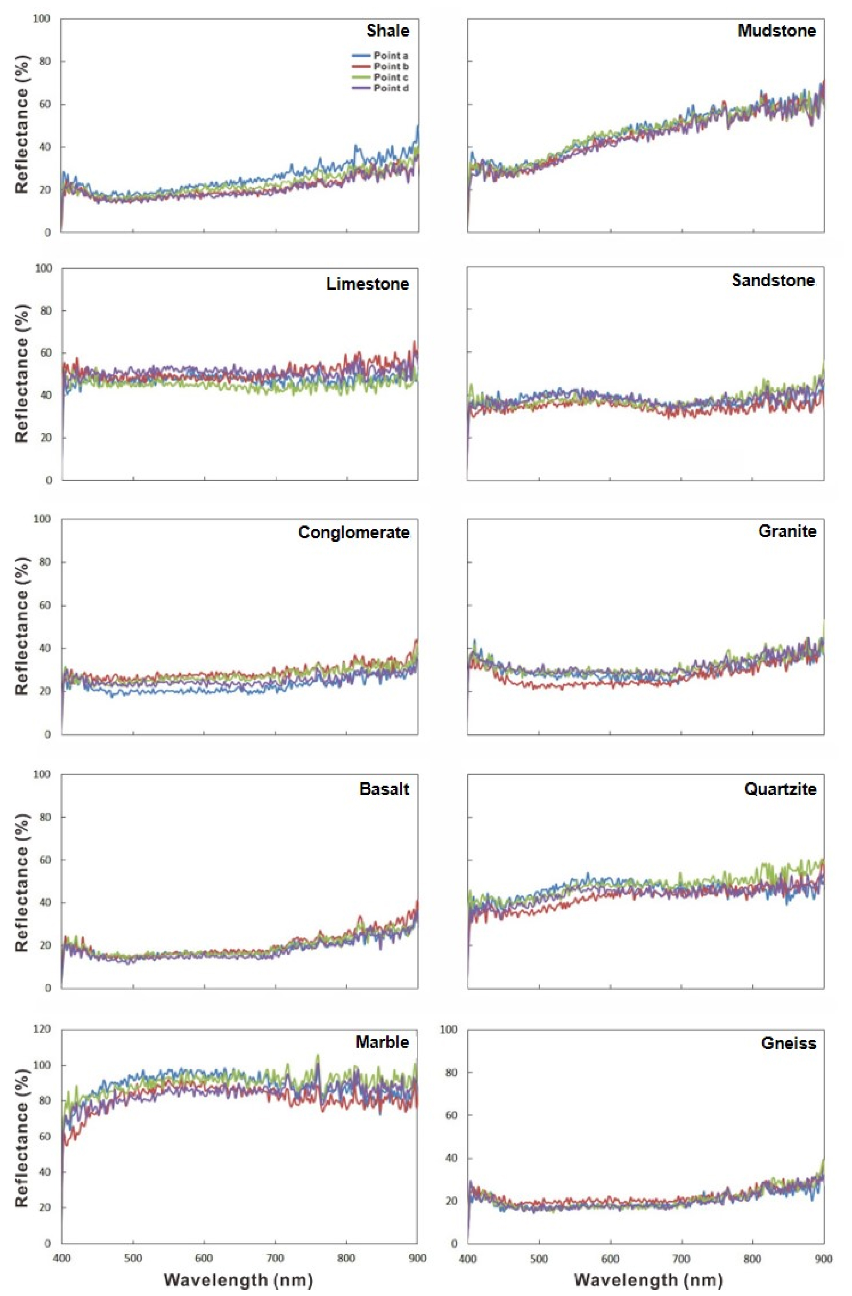
The pattern analysis of the graph showed that shale and conglomerate increased moderately in the visible ray wavelength range and limestone remained at a certain level mudstone is relatively steep. In addition, there are irregular patterns. Sandstone shows a pattern that gradually increases and then decreases. Granite, basalt, and gneiss show a pattern that decreases to approximately 500 nm wavelength and then remains at a certain level. Quartzite increases to approximately 600 nm wavelengths, and marble increases to approximately 500 nm wavelengths and then remained at a certain level (Figs. 7, 8).

In the visible ray range, the reflectance range of four points in limestone, conglomerate, granite, quartzite, and marble is relatively wider than that in shale, mudstone, sandstone, basalt, and gneiss, or there is an irregular gap between each point (Fig. 7). This suggests that the reflectance range is widened owing to the various colors of the matrix and minerals forming the rock or the luster of the surface. Among the rocks used in hyperspectral imaging, limestone is grayish white and conglomerate contains dark red matrixes with various sizes and colors. Because granite is composed of colorless minerals such as white, black, and gray, the range of reflectance of four points is relatively wider than shale, mudstone, sandstone, basalt, and gneiss. Furthermore, quartzite and marble are uniformly colored but have distinct luster, so the reflectance range of the four points is interpreted to be relatively wider than shale, mudstone, sandstone, basalt, and gneiss.

Reflectance Comparison by Wavelength

In this study, wavelengths were divided into visible ray and near infrared ray ranges, and visible rays were divided into blue, green, and red light to compare the reflectance of each range (Table 3). For each wavelength of visible ray (blue, green, and red) 45 reflectance values and 89 reflectance values were used for near infrared rays.

The average reflectance of visible ray range in ten rocks was 16.00~85.78%, the lowest in basalt and the highest in marble. In the near infrared ray range, the average reflectance was 23.94~86.43%, the lowest in basalt and the highest in marble (Table 3). In comparison based on wavelengths in visible ray, basalt was the lowest in blue, red, and green light, and marble was the highest.

The difference in reflectance was shown to be different according to the color of the particles and components constituting the rock. Among the rocks, basalt and gneiss have similar rock gray, and the maximum data value and reflectance data show that basalt was the lowest among the ten rocks with lower value than gneiss. In the case of basalt, a volcanic rock, there is a pore (up to 5~10 mm) formed by the cooling of the lava, which can be interpreted as reflecting less light than the gneiss (a metamorphic rock) without pores, resulting in a lower data value (radiance).

Conclusions

This research on rock spectroscopic information analysis using hyperspectral images aims to perform drone-based hyperspectral imaging on various types of rock samples and compare and classify rocks by analyzing the data obtained. For this purpose, drone-based hyperspectral imaging was performed for ten rocks, and PDV and reflectance, which are intrinsic information of rock, were obtained and compared.

The results of the study showed that there was a difference in the data value and reflectance by rock type, suggesting that the color of the rocks and minerals is varied or the reflectance is different owing to the luster of the surface. Limestone, among the rocks used for hyperspectral imaging, is grayish white, conglomerate contains various sizes and colors in the dark red matrix, and granite is composed of colorless minerals such as white, black, gray, and colored minerals, resulting in a difference in reflectance. In addition, quartzite, and marble are uniformly colored but have distinct luster therefore, the reflectance range of the four points is interpreted to be relatively wider than shale, mudstone, sandstone, basalt, and gneiss. The average reflectance of visible ray range in ten rocks was 16.00~85.78%, the lowest in basalt and the highest in marble. In the near infrared ray range, the average reflectance was 23.94~86.43%, the lowest in basalt and the highest in marble. This is due to the presence of pores in basalt, which possibly caused a difference in reflectance.

Currently, studies for using hyperspectral images for classification and detection of rocks are in the beginning stage, and notably, few studies have been conducted on drone-based hyperspectral image analysis. Therefore, the intrinsic information of rocks obtained through this study will be fully utilized as a basic data for future geological investigation and detection of rocks in extensive areas.