

Introduction
Material and Methods
Concept of SWAT Model
Surface Runoff Calculation
Evapotranspiration Calculation
Groundwater Recharge
Groundwater Recharge (percolation)
Baseflow (groundwater flow)
Data Collection and Study Structure
SWAT Model Enhancement
SWAT-CUP Function
Study Area
Location and Climate
Topography and Land Cover
Measurement of Stream Flow Rate
Result and Discussion
Model Calibration and Validation Using SWAT-CUP
Calibration of Stream Outflow
Comparison of Hydrological Components
Conclusions
Introduction
Accurate simulation of hydrological processes in small watersheds is of crucial importance in water resource management, particularly in regions with scarce data (Arnold et al., 1998; Gassman et al., 2007). Studies of small watersheds are vital in enhancing our understanding of localized hydrological processes and interactions between surface water and groundwater (Guinn Garrett et al., 2012; Eamus et al., 2015). Despite their relatively small size, such watersheds contribute significantly to regional hydrology, local water cycles, flood control, and agricultural productivity (Neitsch et al., 2011; McMillan et al., 2022).
Hydrological modeling, especially in areas with limited data, poses significant challenges. However, previous studies have demonstrated that the soil and water assessment tool (SWAT) can be effectively utilized even in such data-scarce environments. For example, Arnold et al. (1998); McMillan et al. (2012), Moriasi et al. (2012), and Lewis et al. (2018) highlighted the robustness of SWAT in simulating hydrological processes with minimal input data, showcasing its adaptableness in areas with limited observant (McMillan et al., 2012; Moriasi et al., 2012; Lewis et al., 2018). This issue is particularly important for agricultural areas, where precise water management is essential for crop productivity and environmental sustainability (Burger, 2019). Despite these challenges, the SWAT model has proved valuable in simulating hydrological processes including flow generation, due to its flexibility and robustness in handling diverse watershed characteristics (Arnold et al., 1998; Wellen et al., 2015).
Considering these challenges, understanding small watershed dynamics is essential for effective water-resource management, particularly in data-scarce regions. This study focuses on optimizing outflow modeling using the SWAT model for a small watershed, with a methodological approach that addresses constraints imposed by limited discharge data. Accurate forecasting of outflow is critical for applications like flood prediction and sustainable water-use planning (Tan et al., 2020). Given the limited availability of observational data, this study explores novel optimization and calibration techniques, as conventional methods relying on extensive field measurements are impractical (Paradi et al., 2011).
This study addressed these limitations by incorporating indirect indicators, data from regional meteorological stations, flow calculations based on level data, and enhanced calibration procedures to produce reliable flow simulations. This study seeks to develop robust approaches for hydrological modeling in data-limited settings, which are prevalent in rural or underdeveloped watersheds worldwide (Abbaspour et al., 2015), through optimization of SWAT parameters to improve the accuracy and reliability of outflow calculations, while offering insights for effective water-resource management in similar contexts. The novelty of this study lies in the development of a methodological approach for parameter optimization with scarce observation data, leveraging sensitivity analysis and indirect calibration techniques. By advancing our understanding of hydrological modeling in data-scarce environments, this study also establishes a reproducible framework that may be applicable in addressing comparable challenges in other small watersheds.
Material and Methods
Concept of SWAT Model
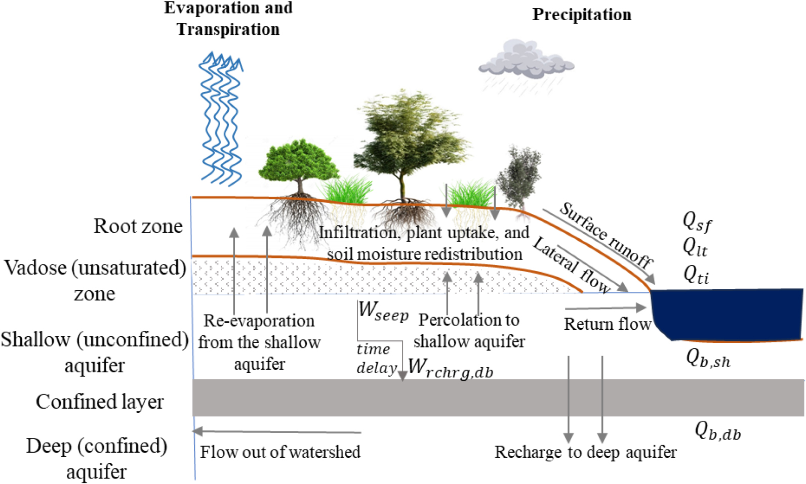
In the SWAT model, water transported through a channel system to gauges comprises four major components: direct surface runoff, Qsf, lateral flow from unsaturated soil profiles, Qlt, drainage from tile systems, Qti, and baseflow originating from underground storage, Qb, as illustrated in Fig. 1, which shows the essential hydrological processes that contribute to outflow conditions. Surface runoff and lateral flow have a direct influence on overall outflow, while infiltration and groundwater recharge dictate the availability of subsurface water. These components influence watershed hydrological balance and outflow characteristics.
SWAT divides underground storage into two components: shallow and deep aquifers. Shallow aquifers receive recharge by percolation through the unsaturated soil profile. To account for the time delay in aquifer recharge after water leaves the soil profile, an exponential-decay weighting function is used (Neitsch et al., 2005). This function is particularly useful in scenarios where recharging from the soil zone to the aquifer does not occur immediately; i.e., typically within 1 day.
Surface Runoff Calculation
Surface runoff was calculated using the soil conservation service (SCS) curve-number method:
where, Q is the surface runoff (mm), P is the rainfall (mm), and S is the potential maximum retention after runoff begins (mm) (Van Liew et al., 2007).
Evapotranspiration Calculation
Evapotranspiration (ET) was estimated using the Penman-Monteith method (Allen et al., 1998):
where, ET is evapotranspiration (mm d-1), Rn is net radiation at crop surface (MJ m-2 d-1), G is soil heat flux density (MJ m-2 d-1), T is mean daily air temperature (°C), u2 is the wind speed at 2 m height (m s-1), es is the saturation vapor pressure (kPa), ea is the actual vapor pressure (kPa), Δ is the slope of the vapor-pressure–temperature curve (kPa °C-1), and γ is the psychrometric constant (kPa °C-1).
Groundwater Recharge
Groundwater recharge is a vital aspect of hydrology, reflecting the volume of water percolating through soil to replenish aquifers. It is calculated using soil water content, field capacity, and saturation levels, as shown:
where, GW is groundwater recharge (mm), SW is soil water content (mm), SAT is soil saturation (mm), and FC is field capacity (mm) (De Vries and Simmers, 2002).
Groundwater Recharge (percolation)
Groundwater recharge, including lateral flow, was estimated using Darcy’s law:
where, Qlat is lateral flow (mm d-1), Ks is hydraulic conductivity (mm d-1), ΔH is the change in the hydraulic head (m), L is the length of the flow path (m), and A is the area (m2) (Costa et al., 2021).
Baseflow (groundwater flow)
Baseflow, Qb, was estimated as follows:
where, Qb is the baseflow at time t (m3 s-1), Qb0 is the initial baseflow (m3 s-1), ALPHA_BF is the Baseflow Alpha Factor (1 d-1), and t is time (d) (Arnold et al., 1998).
Data Collection and Study Structure
The SWAT model was initially used to delineate the watershed into sub-basins using digital elevation models (DEMs), and soil and land-cover data. This defined geographical boundaries and hydrological response units (HRUs), which are unique combinations of soil type, land use, and slope (Arnold et al., 1998). The SWAT model setup included defined hydrological parameters such as the curve number (CN), Manning’s roughness coefficient (n), and SCS parameters. It also involved the specification of groundwater parameters such as the baseflow alpha factor (ALPHA_BF) (Fig. 2). Data collection for stream flow rate involved three methods: flowmeters, weirs, and buoyancy. Using flowmeters, a staff gauge was employed to measure water elevation across the stream. The current water level was recorded at multiple points to calculate the cross-sectional area and velocity. For rectangular weirs, the head of water the height above the weir crest was measured in meters, ensuring precise flow calculations based on standard formulas. The buoyancy method utilized a floating object, such as a water bottle, released at the up and down of the study area cross-section. The time taken for the object to travel a marked distance was recorded, typically over five trials, to determine the average surface velocity. This velocity was then adjusted to estimate the average flow rate. Observations were conducted on three occasions October 9, 14, and 15, 2024 using each method to quantify the flow rate. The data sources for the SWAT model are detailed in Table 1.
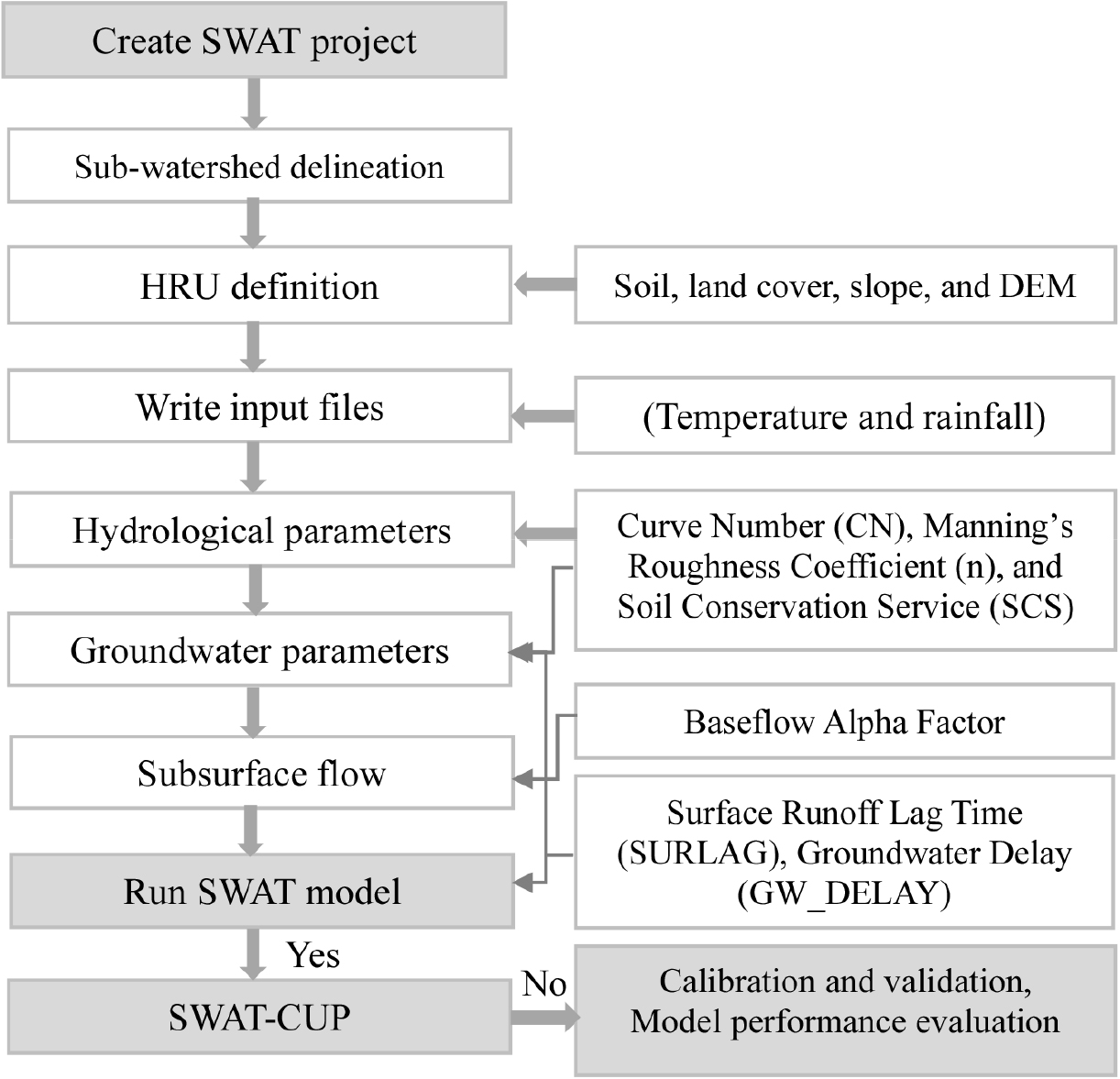
Table 1.
Data categories and sources used in the study
SWAT Model Enhancement
SWAT-CUP Function
SWAT-CUP (calibration and uncertainty procedures) is a tool for the analysis of uncertainty and calibration of the SWAT model to improve its effectiveness. It allows quick calibration, validation, sensitivity analysis, and uncertainty quantification of hydrological models, thereby improving predictive accuracy (Abbaspour et al., 2007). SWAT-CUP uses methods such as SUFI-2 (sequential uncertainty fitting, version 2) to calibrate and quantify uncertainties in hydrological model predictions. It is especially beneficial for calibrating SWAT model parameters to precisely replicate hydrological processes, improving model dependability for water-resource management (Arnold et al., 2010).
The daily streamflow dataset was calibrated and validated using the observed dataset for October 7~16, 2024. On a daily basis, simulated streamflows were compared with measured values and model performance was assessed using Nash-Sutcliffe efficiency (NSE) and Percent Bias (PBIAS) indices (Moriasi et al., 2007).
NSE and PBIAS values were calculated as follows:
where, Oi represents the observed value for daily flow, Pi is the simulated value for daily flow, is the average observed daily flow, and n is the number of daily flow observations.
The NSE index indicates how closely a plot of observed versus simulated values matches the 1 : 1 line, with values ranging from -∞ to 1, with a value of 1 representing optimal model performance. The PBIAS index measures the average tendency of simulated values to be greater or less than observed values. Lower PBIAS values indicate more accurate model simulation, with the ideal value being 0 (Moriasi et al., 2007).
Study Area
Location and Climate
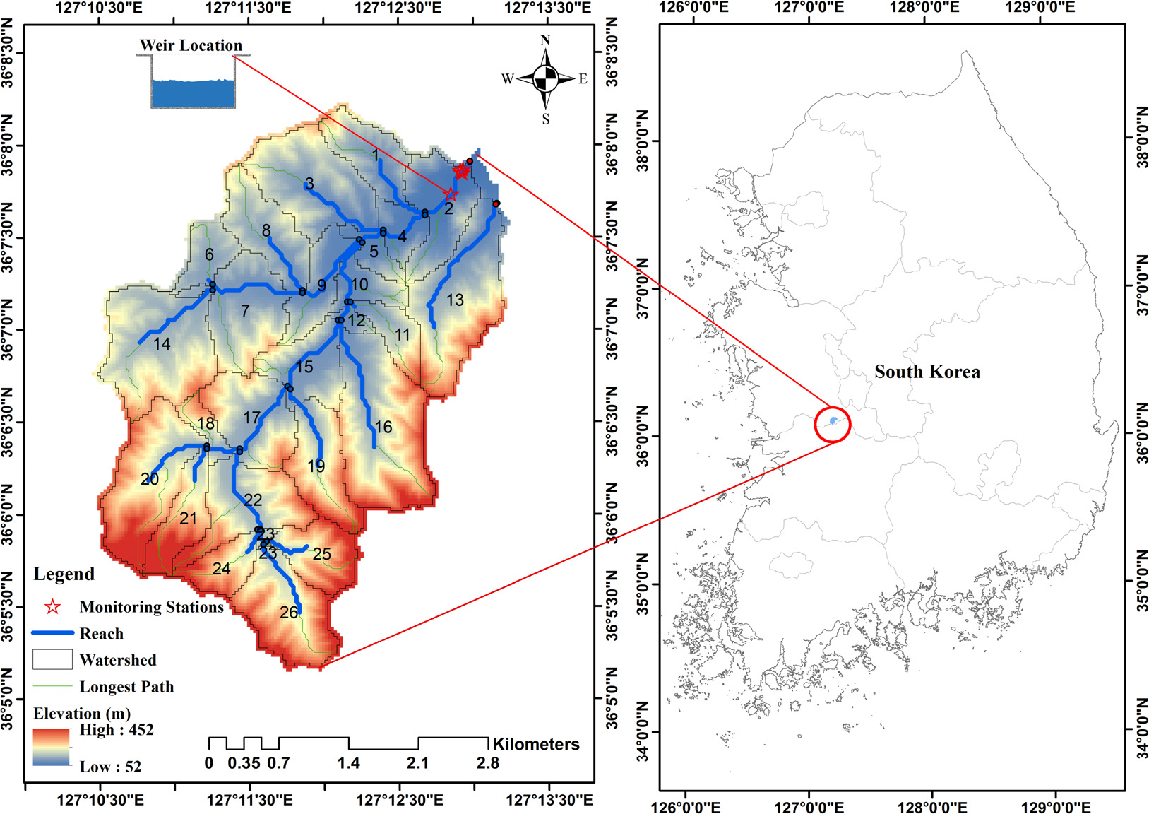
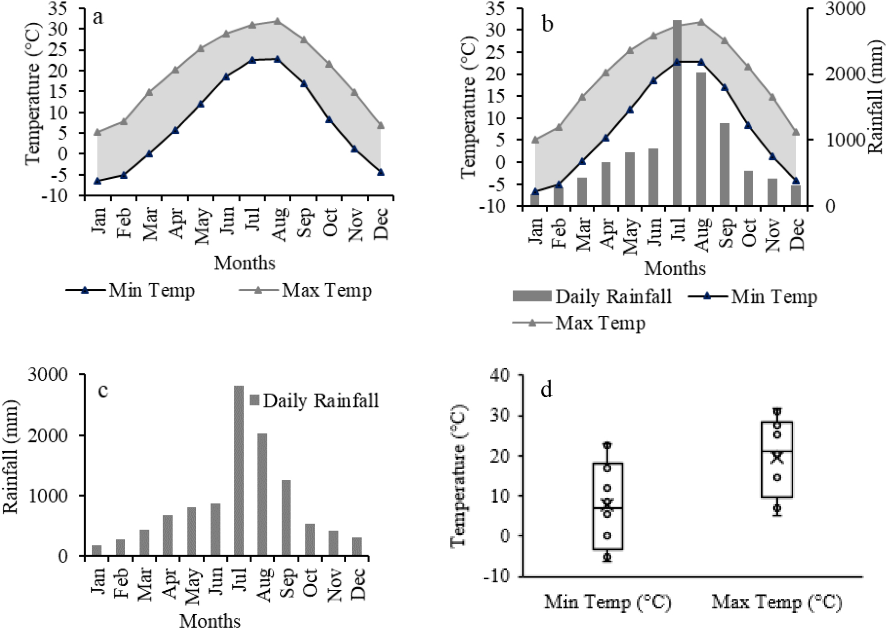
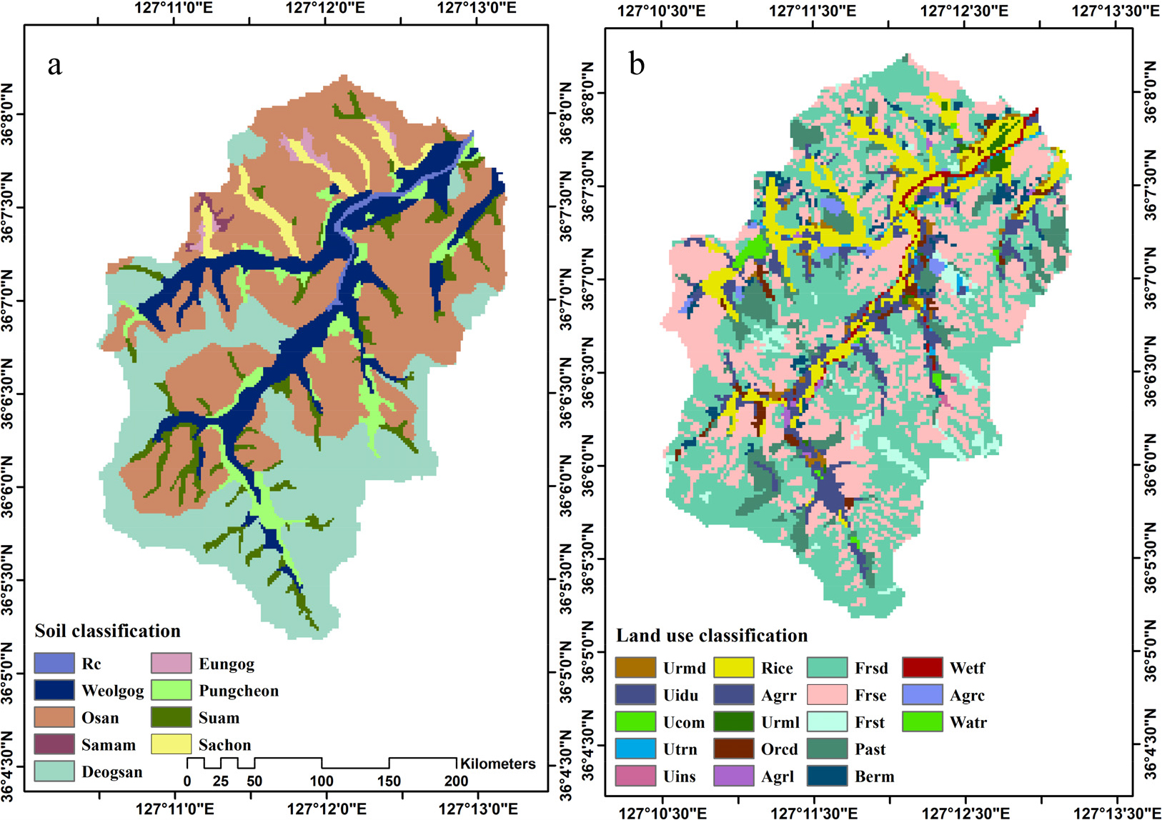
The study area is Seokseo-ri in Nonsan City, Chungcheongnamdo Province, South Korea, covering an area of 14.1 km2 and located at 36.95~37.10°N, 127.10~127.25°E (Fig. 3). The climate of the study area is classified as temperate, with distinct seasons including hot, humid summers and cold, dry winters. The average annual precipitation is 1,481 mm, with most falling during the monsoon season (June~September). Air temperature ranges from an average high of 30°C during summer to an average low of -5°C in winter (Fig. 4a and b). The temperature and rainfall comparison shows rising temperatures and rainfall from January to June, with July peaking at 23 to 31°C and 2,822 mm of rainfall during the monsoon season. rainfall decreases from August to December, with cooler temperatures ranging from -4 to 7°C in December (Fig. 4c). The temperature distribution graph shows the variability in minimum and maximum temperatures throughout the year. minimum temperatures range from around -6 to 23°C, with a median near 10°C, while maximum temperatures range from 5 to 32°C, with a median close to 25°C (Fig. 4d).
The plot highlights greater fluctuations in minimum temperatures, with occasional outliers indicating extreme conditions. Weather stations are located far from the watershed, so the Thiessen polygon approach was used to estimate the rainfall distribution, producing spatially representative precipitation data (Thiessen, 1911). This promoted robust hydrological modeling by increasing the accuracy of rainfall input data for model calibration. These climatic variations significantly influence hydrological processes, affecting evapotranspiration, soil moisture, and surface runoff. Seasonal changes in precipitation and temperature are key factors in determining the hydrological response of the watershed.
Topography and Land Cover
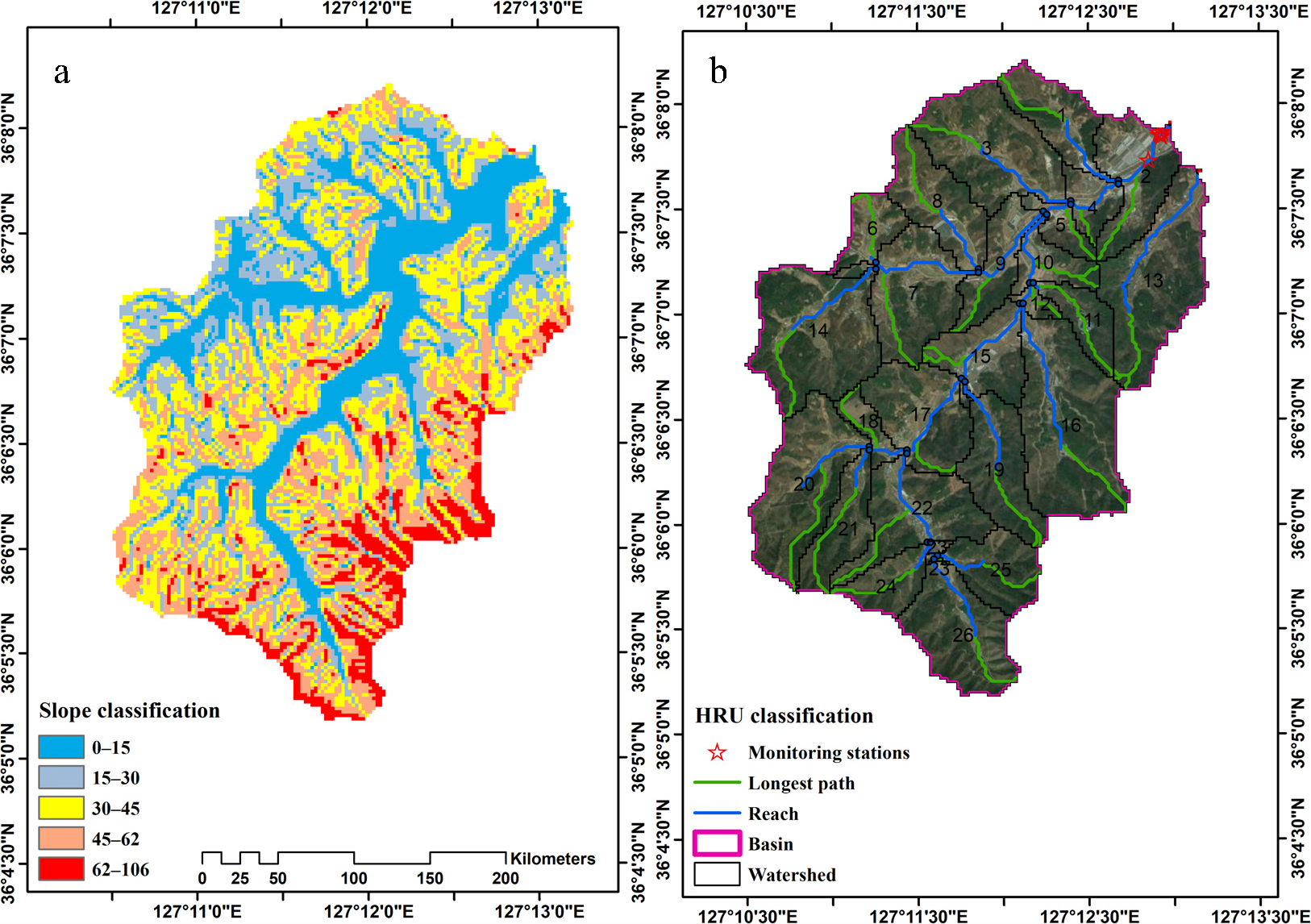
The elevation of the study area ranges from 52 to 452 m above sea level, with substantial topographic diversity. The soil types were reclassified based on the Korean Soil Information System (KSIS) (Hong et al., 2008), and the results are as follows. Osan is the dominant soil type, covering 652.11 ha (46.26% of the watershed), followed by Sachon, which occupies 464.81 ha (32.97%). Samam accounts for 142.80 ha (10.13%), while Suam covers 62.98 ha (4.47%). Other soil types include Deogsan, with 42.90 ha (3.04%), and Eungog, which spans 30.39 ha (2.16%). Smaller contributions come from Weolgog at 5.90 ha (0.42%), Pungcheon at 4.54 ha (0.32%), and Re at 3.33 ha (0.24%) (Fig. 5a). The study area includes diverse land use types, with forest-deciduous (Frsd) being the dominant land use, covering 546.4 ha (38.76% of the watershed). This is followed by forest-evergreen (Frse) at 471.07 ha (33.41%) and rice fields (Rice) at 137.91 ha (9.78%). Other land uses include pasture (Past) at 99.10 ha (7.03%), agricultural land-row crops (Agrr) at 98.51 ha (6.99%), and smaller contributions from residential areas, wetlands, and orchards. The large forested area indicates that natural ecosystems have an important influence in shaping the hydrology of the watershed (Fig. 5b). The slope classification of the study area highlights a diverse topography, ranging from gentle to extremely steep terrain. Gentle slopes (0~15%) cover 159.66 ha (11.33% of the watershed), while moderate slopes (15~30%) span 212.43 ha (15.07%). Steeper slopes (30~45%) account for 298.03 ha (21.14%), and very steep slopes (45~62%) cover 138.04 ha (9.79%). The dominant category is extremely steep terrain (62~106%), which occupies 601.60 ha (42.67%) (Fig. 6a). Watershed characterization entails an outline of hydrological properties such as stream reaches, basin boundaries, and longest flow pathways, which are important in determining the flow network. These slope categories are important to our understanding of hydrological behavior because they influence runoff, erosion potential, and infiltration dynamics, as well as provide critical data for watershed hydrological modeling. Thresholds for land use, soil, and slope were each set at 5%. The model included 827 HRUs, representing unique combinations of land use, soil type, and slope. This allowed for precise simulation of water flow, sediment transport, and nutrient cycling. Additionally, 26 sub-basins were incorporated to effectively represent the watershed’s hydrological processes (Fig. 6b).
Measurement of Stream Flow Rate
As stated in detail in the data collection section, the stream flow rate was measured using flow meters, weirs, and the buoyancy method. The measurements were conducted on three occasions: October 9, 14, and 15, 2024, along the main drainage pathway at its endpoint, designated as the outflow monitoring station, with the weir located near this monitoring station (Fig. 3). These measurements, in conjunction with corresponding groundwater levels, were used to determine the parameter K in the flow-rate estimation equation for a rectangular weir. The flow rate (Q), and coefficient (K) are calculated using the equations:
where, Q is the flow rate (m3 s-1), b is the width of the weir crest (m), h is the head of water above the weir crest (m), and D is the depth of the water channel (m), B is the width of the channel (m).
Stream flow rates were calculated to range between 0.13~0.17 m3 s-1. These formulas provide precise flow-rate estimations by incorporating both weir and channel geometry.
To complement these measurements, a TD-Diver, a highly accurate and durable water level logger, was used to record groundwater levels, pressure, and temperature. The device was installed upstream of the weir (Fig. 3) to record hourly stream water levels from October 7 to 16 and to collect continuous, long-term data, which is essential for validating the simulation outputs. The relationship between these water levels and those recorded during flow-rate measurements was employed to estimate stream flow rates over the entire observation period. Estimated flow rates were in the range of 0.25~0.43 m3 s-1, slightly higher than those measured directly with the velocity meter. The lowest flow rate of 0.25 m3 s-1 occurred on October 13, a day without rainfall, and the highest of 0.43 m3 s-1 on October 8, following rainfall with increased surface runoff. These results underscore the influence of rainfall events on streamflow dynamics and explain flow-rate variability within the 10-day observation period. The combination of intermittent and continuous measurements thus provided a robust approach to assessing streamflow variability and its response to hydrological events.
Result and Discussion
Model Calibration and Validation Using SWAT-CUP
The SWAT-CUP tool was used to calibrate and validate the SWAT model by adjusting model parameters to improve consistency between simulated and observed streamflow data (Table 2). This tool provides an interface for automatic calibration, aiding the minimization of model uncertainty and enhancing model accuracy (Abbaspour et al., 2007). The calibration process involved both trial and error and reference values from existing literature. Initial values for the model parameters were based on typical values reported in the literature for similar hydrological and geographical settings. The SWAT-CUP tool was then used to fine-tune these parameters, adjusting them iteratively to reduce discrepancies between simulated and observed streamflow data.
Table 2.
Calibrated SWAT-CUP model parameters for the study area
The adjustments for specific parameters were based on a combination of factors:
• The Curve Number (CN2) was increased from 58 to 75, indicating a moderate runoff potential. This modification was shown by studies in similar areas (Garg et al., 2013; Sadiqi et al., 2024), which recommend that such values are common for watersheds with similar soil properties and land cover.
• Available Water Capacity (SOL_AWC) was calibrated as 0.42, which is higher than the typical values for the area but was chosen to reflect the high soil-moisture retention capacity, particularly given the importance of sustaining soil moisture during dry periods for local agriculture (Lee et al., 2019; Moon et al., 2024).
• Saturated Hydraulic Conductivity (SOL_K) was calibrated as 0.91 mm h-1, which is constant with the loamy soils in the area. The value was used based on local soil characteristics and data from similar work in agricultural watersheds (Sadiqi et al., 2024).
• Baseflow Alpha Factor (ALPHA_BF) was reduced from 0.1 to 0.08, representing a low contribution of groundwater to streamflow, consistent with local geological characteristics and prior studies (Abbaspour et al., 2007; Lee et al., 2019).
• Groundwater Delay Time (GW_DELAY) was calibrated as 250 days, implying a long delay in groundwater contributing to streamflow. This is consistent with local hydrogeology, where the presence of thick clay layers hinders groundwater movement, with the delayed response being crucial for sustaining baseflow during prolonged dry periods (Lee et al., 2019).
• Surface Runoff Lag-time (SURLAG) was set to 1.71 h, implying a rapid response to high-intensity rainfall and reflecting the steep topography and relatively low infiltration capacity of much of the watershed. Rapid runoff also indicates flash-flood potential, especially during the monsoon season, which requires effective runoff management strategies (Moon et al., 2024).
Calibration results indicate that the watershed has a high infiltration capacity with a persistent baseflow component, which helps maintain streamflow during dry periods. However, a CN2 value of 75 and a SURLAG value of 1.71 h indicate a tendency for rapid runoff after high-intensity rains, which raises the possibility of peak-flow events, possibly leading to flash floods. These findings are consistent with those of similar studies of other watersheds in South Korea (e.g., Garg et al., 2013), which have highlighted the relevance of runoff management and soil-water interactions in regions with similar climatic and topographic conditions.
Calibration of Stream Outflow
SWAT model calibration for streamflow indicated a close alignment between predicted and monitored precipitation, particularly concerning seasonal flow dynamics and precipitation events, as shown in Fig. 7. The model effectively captured responses to rainfall events, with simulated flow peaks corresponding to periods of high precipitation, thereby highlighting model robustness.
Seasonal variations in simulated streamflow and daily precipitation are highlighted in Fig. 7. Precipitation is low during January~March, typically at <50 mm d-1, with limited streamflow. Precipitation increases during April~June, to 100 mm d-1, with the simulated flow rising in response at the start of the rainy season, which peaks in July~August with daily precipitation of up to 200 mm and significant increases in streamflow, to the highest flow-rates of the year. After the peak, rainfall declines in September~October, but streamflow remains high due to delayed runoff. Finally, during November~December, precipitation falls to <50 mm d-1, with flow rates returning to levels like those of the dry season. Fig. 7 thus portrays the seasonal dynamics of precipitation and streamflow, with peak flows during the wettest months. A previous study (Lee et al., 2024) has shown that longer observational periods and improved spatial coverage of meteorological data allow more precise calibration and simulation of hydrological processes. However, the SWAT model was performed effectively here, reflecting its ability to accurately recreate streamflow dynamics in response to seasonal rainfall patterns, even with limited field data.
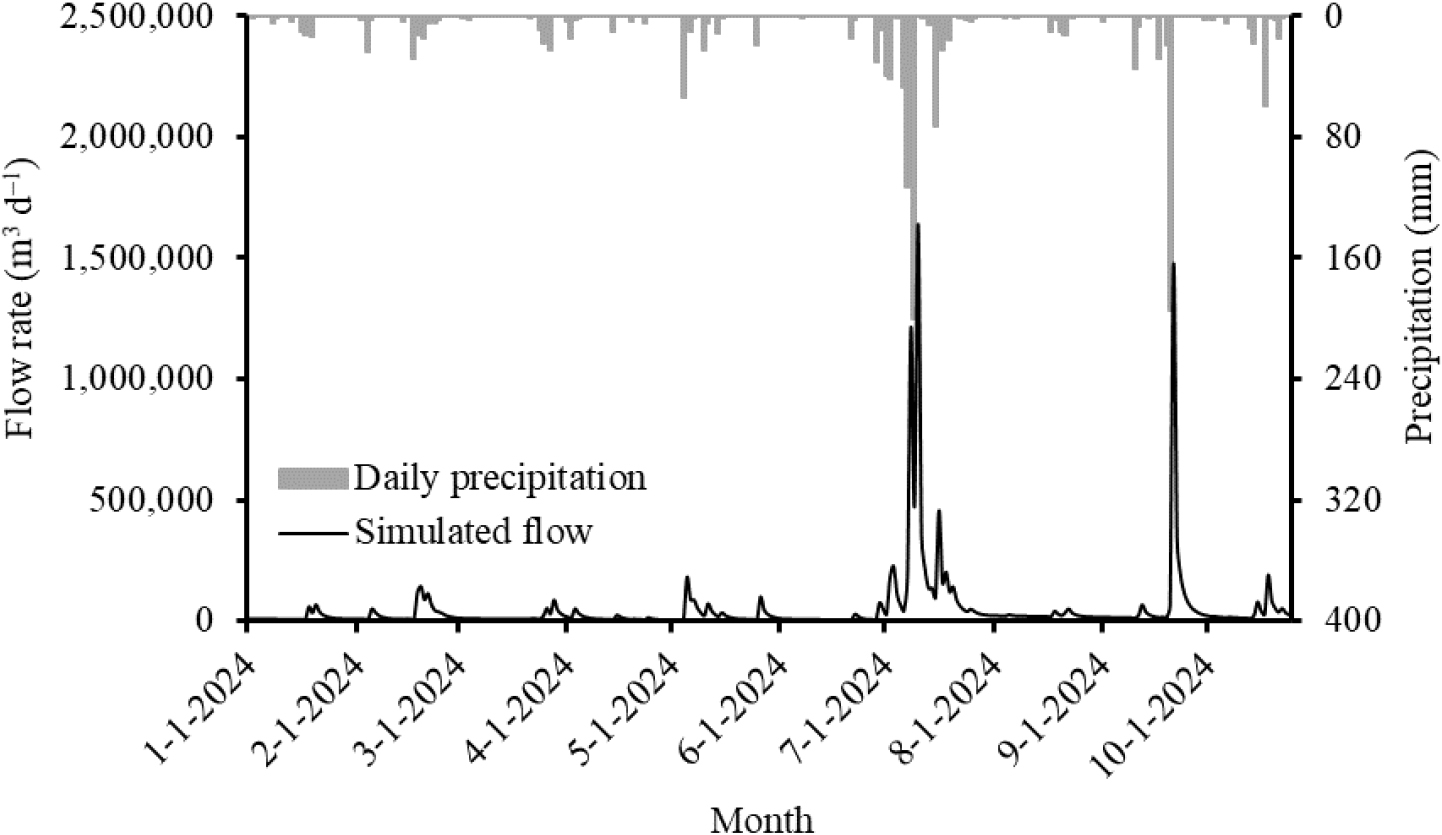
Fig. 8 provides a comparison of flow-rate data for October 7~16 (2024) between SWAT modeling, TD-diver measurements, and field measurements for the monitored stream stations in the study area. During this period, simulated flow rates remained relatively uniform at ~0.2 m3 s-1, while calculated levels varied in the range of 0.25~0.43 m3 s-1 and measured flow rates within 0.13~0.17 m3 s-1. The graph indicates a very close agreement between observed and simulated flow rates, with R2 = 0.97, demonstrating a very strong correlation between the values on October 7, 10, and 13, 2024 (Fig. 8). This comparison highlights the reliability of the SWAT model and field measurements in capturing flow dynamics.
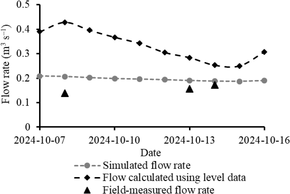
Any mismatch between observed, calculated, and simulated flow rates may be attributed to several key factors, as follows. The weir for flow measurement was located 150 m upstream of the SWAT outlet, with the modeled watershed therefore covering a larger area, with higher simulated flow rates. Flow measurements at the weir, based on water-level sensors, may introduce errors in elevation, affecting the accuracy of calculations. SWAT simplifies information on land use, soil properties, and topography, while observed data reflect localized conditions, creating discrepancies. Localized rainfall and microclimatic effects are often missed in SWAT input data, leading to runoff errors. Calculated field data, recorded hourly, may also differ from daily SWAT time steps, which may fail to capture small variations in flow. Seasonal differences further complicate the comparison, with about 70% of precipitation occurring during the wet season, with sharp transitions to dry periods; observations capture such variations better than averaged SWAT seasonal variations. Finally, observed flows may be attenuated or delayed due to natural storage processes associated with groundwater movement, while SWAT often predicts more rapid runoff due to simplified hydrological processes.
Despite these limitations, overall trends indicate a positive correlation between outputs, with the SWAT model generally capturing flow dynamics well. Studies in other watersheds (Lee et al., 2024; Sadiqi et al., 2024) have shown that accurate calibration of parameters such as CN2 and SURLAG improves the simulation of runoff events and flow peaks. For October 2024 there was a significant correlation (R2 = 0.97) between field-measured and simulated flow rates, with the SWAT model closely matching observed data. However, the PBIAS for field-measured flow rate was -13.6%, indicating that simulated flow rates tend to underestimate streamflow relative to field observations. However, the model performs satisfactorily, with an NSE value of 0.54 for October 2024, implying acceptable accuracy, though with room for improvement. The PBIAS value further reflects this, indicating that while the model underestimated streamflow, its performance remained within acceptable limits during the calibration period.
Comparison of Hydrological Components
The hydrological analysis highlighted water-flow dynamics, focusing on rainfall, surface runoff, evapotranspiration, lateral flow, and groundwater recharge, and showing seasonal and annual fluctuations in the water budget.
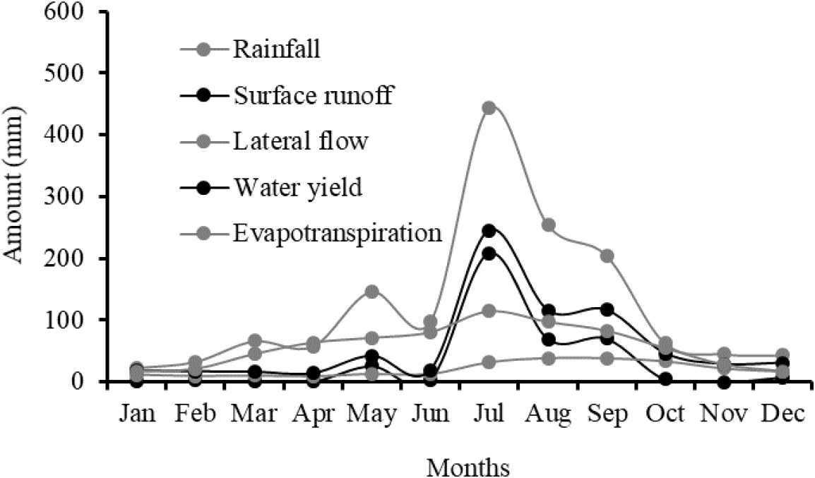
Monthly variations in hydrological components during 2021~2024 are shown in Fig. 9, with peak values observed during summer, particularly in July. The average monthly rainfall from 2021 to 2024 reached its maximum of ~450 mm in July, driving significant increases in surface runoff (120 mm), water yield (380 mm), lateral flow (39 mm), and evapotranspiration (115 mm). Lateral flow values ranged from 9.3 mm in April to a peak of 38.9 mm in August, indicating greater subsurface movement during wetter months. Evapotranspiration also followed a seasonal trend, peaking at 115 mm in July due to high temperatures and vegetation growth, and dropping to ~17 mm in January and December.
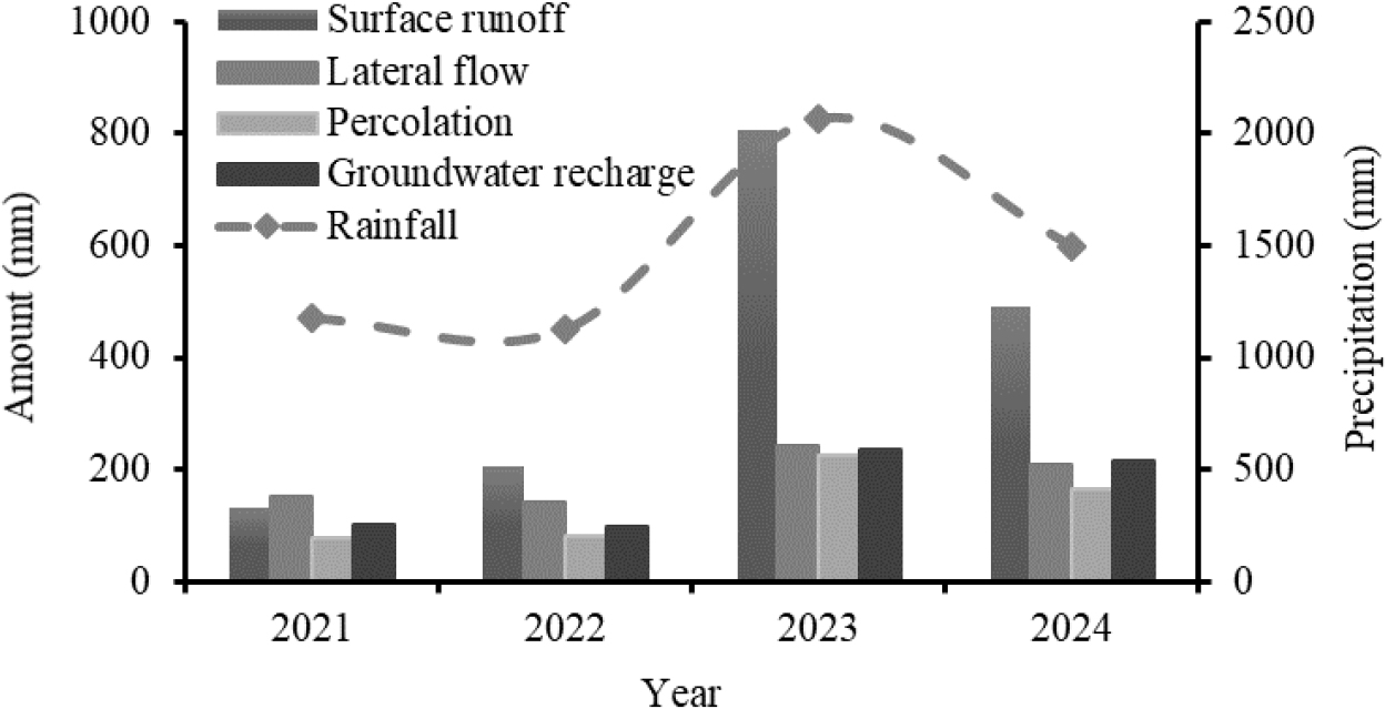
The variability of hydrological components during 2021~2024 is highlighted in Fig. 10, driven by differences in annual precipitation. In 2023, the wettest year, total precipitation was ~2,000 mm, leading to significant increases in surface runoff (806 mm) and groundwater recharge (236 mm). In contrast, during the drier year of 2022, with 1,127 mm of precipitation, surface runoff decreased to 206 mm, and groundwater recharge dropped to 98 mm. Over the four years, annual precipitation averaged 1,480 mm, with surface runoff contributing 397 mm annually including percolation of 137 mm and groundwater recharge of 175 mm. The total estimated annual outflow, including lateral flow of 249 mm, was 711 mm, representing ~48% of the total precipitation.
Our analysis provides useful information concerning the water budget in the study area. The observed surge in surface runoff and lateral flow during the summer months is indicative of the monsoon influence, which is common in regions such as South Korea. This aids our understanding of how rainfall patterns influence water-balance components. High evapotranspiration throughout the summer months reflects greater warmth and vegetation activity, consistent with seasonal fluctuation in water flows, as observed in other Korean watersheds, with monsoon-driven precipitation having a significant impact on annual water availability and hydrological responses (Kim et al., 2022; Lee et al., 2024).
Our findings also support the concept of water balance, with inflow (precipitation) being balanced by outflow (runoff, evapotranspiration, and groundwater recharge). The high reactivity of the watershed to rainfall events, as indicated by peak flow components during the monsoon, highlights that appropriate management methods are required to mitigate flooding and improve water consumption during dry seasons.
Conclusions
The SWAT model with SWAT-CUP calibration was used in this study of a small watershed in South Korea. The SWAT-CUP results indicate that parameters such as Curve Number (CN2), Surface Runoff Lag-time (SURLAG), and the Baseflow Alpha Factor (ALPHA_BF) are more sensitive than the other parameters, meaning that fine-tuning them during calibration is crucial for achieving accurate simulation results. Other parameters, while still important, have less influence on the modeled outputs compared to these three. The streamflow simulations were consistent with observed values (R2 = 0.97) during October 7~16, 2024.
The analysis of water-flow components for 2021~2024 highlights similar patterns for surface runoff, percolation, lateral flow, and groundwater recharge. Surface runoff ranged over 206~806 mm per year, with a considerable response to precipitation, especially during the peak rainfall season. Monthly outflow data show peaks in summer months, of up to 120 mm, depending on precipitation events.
Percolation estimates of 80~230 mm yr-1 indicate that a significant portion of precipitation infiltrates the soil, promoting groundwater recharge, consistent with SOL_K and SOL_AWC values of 0.9 mm h-1 and 0.42, respectively, again indicating moderate to high infiltration potential. Lateral flow remained steady at ~220 mm yr-1, while groundwater recharge ranged over 109~236 mm yr-1, contributing positively to baseflow, especially during drier periods. The observed versus simulated streamflow indicates a strong correlation (R2 = 0.97). ALPHA_BF and GW_DELAY values of 0.08 and 250 d were critical in accurately simulating groundwater discharge, with consistent baseflow throughout the year supporting water availability during dry seasons.
Streamflow peaked in summer, with precipitation reaching ~450 mm from 2021 to 2024. In contrast, winter and spring had much less precipitation, with outflow reflecting the lower intake. Our findings may aid water-resource management of the watershed by precisely estimating streamflow and balancing runoff, baseflow, and recharge, thereby laying the groundwork for informed decisions concerning flood risks and improvement of water availability during dry years.
